Korb K.B., Nicholson A.E. Bayesian Artificial Intelligence
Подождите немного. Документ загружается.

nomial Parameterization Algorithm 7.1 requires the specification of priors for the
parameters, including an equivalent sample size which implicitly records a degree of
confidence in those parameters. Also,
8.6.3 shows how prior probabilities for arc
structure can be fed into the learning process. And, indeed, this section relies upon
an understanding of those sections. The difference is one of intent and degree: in
those chapters we were concerned with specifying some constraints on the learning
of a causal model; here we are concerned with modifying a model already learned
(or elicited).
9.4.1 Adapting parameters
We describe how to modify multinomial parameters given new complete joint obser-
vations. This can be done using the Spiegelhalter-Lauritzen Algorithm 7.1 under the
same global and local assumptions about parameter independence. Recall that in that
process the prior probabilities for each parameter are set with a particular equivalent
sample size. If the parameters have actually been learned with some initial data set,
then subsequent data can simply be applied using the same algorithm, starting with
the new equivalent sample size and Dirichlet parameters set at whatever the initial
training has left. If the parameters have been elicited, then you must somehow es-
timate your, or the expert’s, degree of confidence in them. This is then expressed
through the equivalent sample size, the larger the sample size the greater the confi-
dence in the parameter estimates and the slower the change through adapting them
with new data.
Suppose for a particular Dirichlet parameter
the expert is willing to say she
gives a 90% chance to the corresponding probability
lying within the inter-
val
. The expected value (i.e., the mean) of the Dirichlet distribution over state
corresponds to the estimated parameter value:
where is the equivalent sample size. The variance over state of the
Dirichlet distribution is:
The 90% confidence interval of this distribution lies within 1.645 standard deviations
of the mean and is
We can solve this algebraically for values of and that yield the mean and 90%
confidence interval. A solution is an equivalent sample size
and a parameter
value
of 3.
Of course, when this procedure is applied independently to the different Dirichlet
parameters for a single parent instantiation the results may not be fully consistent. If
© 2004 by Chapman & Hall/CRC Press LLC

the expert reports the above interval for the first state of the binary child variable and
for the second, then the latter will lead to an equivalent sample size of
and . Since the equivalent sample size applies to all of the values of the
child variable for a single instantiation, it cannot be both 15 and 24! The sample size
must express a common degree of confidence across all of the parameter estimates
for a single parent instantiation. So, the plausible approach is to compromise, for
example, taking an average of the equivalent sample sizes, and then finding numbers
as close to the estimated means for each state as possible. Suppose in this case, for
example, we decide to compromise with an equivalent sample size of 20. Then the
original probabilities for the two states, 0.2 and 0.5, yield
, which does
not work. Normalizing (with round off) would yield instead
.
When parameters with confidence intervals are estimated in this fashion, and are
not initially consistent, it is of course best to review the results with the expert(s)
concerned.
Fractional updating is what Spiegelhalter and Lauritzen[263] call their technique
for adapting parameters when the sample case is missing values, i.e., for incomplete
data. The idea is simply to use the Bayesian network as it exists, applying the values
observed in the sample case and performing Bayesian propagation to get posterior
distributions over the unobserved cases. The observed values are used to update the
Dirichlet distributions for those nodes; that is, a 1 is added to the relevant state pa-
rameter for the observed variable. The posteriors are used to proportionally update
those variables which were unobserved; that is,
is added to the state parameter
corresponding to a value which takes the posterior
. The procedure is complicated
by the fact that a unique parent instantiation may not have been observed, when
the proportional updating should be applied across all the possible parent instanti-
ations, weighted by their posterior probabilities. This procedure unfortunately has
the drawback of overweighting the equivalent sample size, resulting in an artificially
high confidence in the probability estimates relative to new data.
Fading refers to using a time decay factor to underweight older data exponentially
compared to more recent data. If we fade the contribution of the initial sample to
determining parameters, then after sufficient time the parameters will reflect only
what has been seen recently, allowing the adaptation process to track a changing
process. A straightforward method for doing this involves a minor adjustment to the
update process of Algorithm 7.1 [128, pp. 89-90]: when state
is observed, instead
of simply adding 1 to the count for that state, moving from
to , you first
discount all of the counts by a multiplicative decay factor
.Inotherwords
the new Dirichlet distribution becomes
. In the limit,
the Dirichlet parameters sum to
, which is called the effective sample size.
9.4.2 Structural adaptation
Conceivably, rather than just modifying parameters for an existing structure, as new
information comes to light we might want to add, delete or reverse arcs as well.
Jensen reports that “no handy method for incremental adaptation of structure has
been constructed” [128]. He suggests the crude, but workable, approach of accumu-
© 2004 by Chapman & Hall/CRC Press LLC

lating cases and rerunning structure learning algorithms in batch mode periodically.
In addition to that, the Bayesian approach allows for structural adaptation, at least
in principle. If we let what has previously been learned be reflected in our prior prob-
abilities over structures, then new data will update our probability distributions over
causal structure. That simply is Bayesian theory. To be sure, it is also Bayesian up-
dating without model selection, since we need to maintain a probability distribution
over all of the causal structures that we care to continue to entertain. A straightfor-
ward implementation of such inference will almost immediately be overwhelmed by
computational intractability.
However, there is a simpler technique available with CaMML for structural adap-
tation. Since CaMML reports its estimate of the probability of each directed arc at
the end of its sampling phase, and since CaMML allows the specification of a prior
probability for such arcs before initiating causal discovery, those probabilities can be
reused as the prior arc probabilities when performing learning with new data. This
is crude in that there is no concept of equivalent sample size operating here; so there
is no way to give greater weight to the initial data set over the latter, or vice versa.
Nevertheless, it can be an effective way of adapting previously acquired structure.
9.5 Summary
There is an interplay between elements of the KEBN process: variable choice, graph
structure and parameters. Both prototyping and the spiral process model support this
interplay. Various BN structures are available to compactly and accurately represent
certain types of domain features. While no standard knowledge engineering process
exists as yet, we have sketched a framework and described in more detail methods
to support at least some of the KE tasks. The integration of expert elicitation and
automated methods, in particular, is still in early stages. There are few existing tools
for supporting the KEBN process, although some are being developed in the research
community, including our own development of VE and Matilda.
9.6 Bibliographic notes
An excellent start on making sense of software engineering is Brooks’ Mythical Man-
Month [33]. Sommerville’s text is also worth a read [261]. You may also wish
to consult a reference on software quality assurance in particular, which includes
detailed advice on different kinds of testing [93].
Laskey and Mahoney also adapt the ideas of prototyping and the spiral model to
the application of Bayesian networks [166]. Bruce Marcot [182] has described a
© 2004 by Chapman & Hall/CRC Press LLC

KEBN process for the application area of species-environment relations.
One introduction to parametric distributions is that of Balakrishnan and Nevzorov
[14]. Mosteller et al.’s Statistics by Example [196] is an interesting and readily ac-
cessible review of common applications of different probability distributions. An
excellent review of issues in elicitation can be found in Morgan and Henrion’s Un-
certainty [194], including the psychology of probability judgments.
9.7 Problems
Problem 1
The elicitation method of partitioning to deal with local structure is said in the text to
directly correspond to the use of classification trees and graphs in Chapter 7. Illus-
trate this for the Flu, Measles, Age, Fever example by filling in the partitioned CPT
with hypothetical numbers. Then build the corresponding classification tree. What
do partition elements correspond to in the classification tree?
Problem 2
Consider the BN that you constructed for your own domain in Problem 5, Chapter 2.
(Or if you haven’t completed this problem, use an example network from elsewhere
in this text, or one that comes with a BN software package.)
1. Identify the type of each node: target/query, evidence/observation, context,
controllable.
2. Re-assess your choice of nodes and values, particularly if you discretized a
continuous variable, in the light of the discussion in
9.3.1.
3. Label each arc with the relationship that is being modeled, using the relation-
ships described in
9.3.2 or others you might think of.
4. Use Matilda to investigate the dependence and independence relationships in
your network.
5. Can you map the probabilities in the CPTs into a qualitative scale, as in
9.3.3.2?
Problem 3
Using some of methods from this chapter, reengineer one of the BN applications you
developed for one of the problems from Chapter 5. That is, redo your application, but
employ techniques from this chapter. Write up what you have done, with reference
to specific techniques used. Also, describe the difference use of these techniques has
made in the final BN.
© 2004 by Chapman & Hall/CRC Press LLC

10
Evaluation
10.1 Introduction
Critical to developing Bayesian networks is evaluative feedback. One of the major
advantages of the spiral, prototyping development of software is that from the very
beginning a workable (if limited) user interface is available, so that end-users can get
involved in experimenting with the software and providing ideas for improvement.
This is just as true with the knowledge engineering of Bayesian networks, at least
when a GUI front-end is available.
In this chapter we discuss some of the formal and semi-formal methods of gener-
ating evaluative feedback on Bayesian models. The first three types of evaluation are
largely concerned with obtaining feedback from human experts, using an elicitation
review process, sensitivity analysis and the evaluation of cases. The last section in-
troduces a number of formal metrics for evaluating Bayesian models using statistical
data.
10.2 Elicitation review
An elicitation review is a structured review of the major elements of the elicitation
process. It allows the knowledge engineer and domain expert to take a global view of
the work done and to check for consistency. This is especially important when work-
ing with multiple experts or combining expert elicitation with automated learning
methods.
First, the variable and value definitions should be reviewed, encompassing:
1. A clarity test: do all the variables and their values have a clear operational
meaning — i.e., are there definite criteria for when a variable takes each of
its values? “Temperature is high” is an example that does not pass the clarity
test
; this might be refined to “Temperature 30 degrees” which does.
2. Agreement on variable definitions:
Are all the relevant variables included? Are they named usefully?
We have been guilty of exactly this in 3.2.
© 2004 by Chapman & Hall/CRC Press LLC
Are all states (values) appropriate? Exhaustive and exclusive?
Are all state values useful, or can some be combined?
Are state values appropriately named?
Where variables have been discretized, are the ranges appropriate?
3. Consistency checking of states: are state spaces consistent across different
variables? For example, it might cause misunderstanding if a parent variable
takes one of the values
veryhigh, high, medium, low and its child takes one
of
extremelyhigh, high, medium, low .
The graph structure should be reviewed, looking at the implications of the d-
separation dependencies and independencies and at whether the structure violates
any prior knowledge about time and causality. A review of local model structure
based on partitions or classification trees may also be conducted.
Reviewing the probabilities themselves can involve: comparing elicited values
with available statistics; comparing values across different domain experts and seek-
ing explanation for discrepancies; double-checking cases where probabilities are ex-
treme (i.e., at or close to 0 or 1).
It is often useful to do a model walk-through, where a completed version of the
model is presented to domain experts who have not been involved in the modeling
process to date. All components of the model are evaluated. This can be done by
preparing a set of cases with full coverage of the BN — i.e., sets of assumed observa-
tions with various sets of query nodes, when the reasoning required exercises every
part of the network. This performs a similar function to code reviews in the software
engineering process.
10.3 Sensitivity analysis
Another kind of evaluation is to analyze how sensitive the network is to changes in
parameters or inputs; this is called sensitivity analysis. The network outputs may
be either the posterior probabilities of the query node(s) or (if we are building a
decision network) the choice of action. The changes to be tested may be variations
in the evidence provided, or variations in the network parameters — specifically
conditional probability tables or utilities. We will look at each of these types of
changes in turn.
10.3.1 Sensitivity to evidence
Earlier in 9.3.2.2, we saw how the properties of d-separation can be used to de-
termine whether or not evidence about one variable may influence belief in a query
variable. It is also possible to measure this influence. Given a metric for changes in
© 2004 by Chapman & Hall/CRC Press LLC
belief in the query node (which we address just below), we can, for example, rank
evidence nodes for either the maximum such effect (depending on which value the
evidence node takes) or the average such effect. It is also possible, of course, to
rank sets of evidence nodes in the same way, although the number of such sets is
exponential in the number of evidence nodes being considered. In either case, this
kind of sensitivity analysis provides guidance for the collection of further evidence.
An obvious application area for this is medical diagnosis, where there may be multi-
ple tests available; the clinician may like to perform the test that most decreases the
uncertainty of the diagnosis.
So, how to quantify this uncertainty? What metric of change should we employ?
We would like to drive query node probabilities close to 0 and 1, representing greater
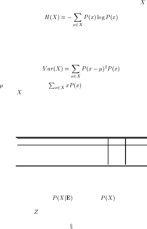
certainty. Entropy is the common measure of how much uncertainty is represented
in a probability mass. The entropy of a distribution over variable
is (cf. Defini-
tion 8.2):
(10.1)
For continuous variables, we can simply substitute integration for summation. The
goal, clearly, is to minimize entropy: in the limit, entropy is zero if the probability
mass is concentrated on a single value.
A second measure used sometimes is variance:
(10.2)
where
is the mean, i.e., . Variance is the classic measure of the
dispersion of
around its mean. The greater the dispersion, the less is known;
hence, we again aim to reduce this measure to zero.
TABLE 10.1
Entropy and variance measures for three distributions
(H is computed with natural logs)
P(Z=1) P(Z=2) P(Z=3) P(Z=4) H(Z) Var(Z)
10000.0 0.0
0.25 0.25 0.25 0.25
1.39 1.25
00.50.500.69 0.25
Whether using entropy or variance, the metric will actually be computed for the
query node conditional upon whatever evidence nodes are being tested for sensitivity
— that is, for the distribution
rather than . To provide a feel for these
measures, Table 10.1 compares the entropy and variance for a few distributions over
a quaternary variable
.
The main BN software packages provide a facility to quantify the effect of evi-
dence using some such measure (see
B.4).
© 2004 by Chapman & Hall/CRC Press LLC

TABLE 10.2
Output from Netica’s sensitivity to findings function for
the Cancer Example, with
as the query node
Node value min max Entropy (%)
of Bel(C) Bel(C) Reduction
No evidence. Bel(C=T)=0.012
C T 0 1 0.0914 100%
F 0 1
X T 0.001 0.050 0.0189 20.7%
F 0.950 0.999
S T 0.003 0.032 0.0101 11.0%
F 0.968 0.997
D T 0.006 0.025 0.0043 4.7%
F 0.975 0.994
P T 0.001 0.029 0.0016 1.7%
F 0.971 0.990
Evidence . Bel(C=T)=0.050
C T 0 1 0.2876 100%
S T 0.013 0.130 0.0417 14.5%
D T 0.026 0.103 0.0178 6.2%
P T 0.042 0.119 0.0064 2.2%
Evidence , . Bel(C=T)=0.129
C T 0 1 0.5561 100%
D T 0.069 0.244 0.0417 7.5%
P T 0.122 0.3391 0.0026 0.47%
Evidence , , . Bel(C=T)=0.244
C T 0 1 0.8012 100%
P T 0.232 0.429 0.0042 0.53%
Lung cancer example
Let us re-visit our lung cancer example from Figure 2.1 to see what these measures
can tell us.
is our query node, and we would like to know observations
of which single node will most reduce uncertainty about the cancer diagnosis. Ta-
ble 10.2 shows the output from the Netica software’s “sensitivity to findings” func-
tion, which provides this information. Each pair of rows tells us, if evidence were
obtained for the node in column 1:
The minimum (column 3) and maximum (column 4) posterior probabilities for
or (column 2); and
The reduction in entropy , both in absolute terms (column 5) and as a percent-
age (column 6).
The first set of results assumes no evidence has been acquired, with the prior
. As we would expect, all the “min” beliefs are less than
the current belief and “max” beliefs above. Obtaining evidence for
itself is a
degenerate case, with the belief changing to either 0 or 1. Of the other nodes,
© 2004 by Chapman & Hall/CRC Press LLC
(XRay) has the most impact on
,then , and respectively. Netica’s output
does not tell us which particular observed value actually gives rise to the minimum
and maximum new belief; however, this is easy to work out.
Suppose that the medical practitioner orders the test having the most potential
impact, namely an X-ray, which then returns a positive result. The second set of
results in Table 10.2 shows the new sensitivity to findings results (with values for
omitted). In this example the relative ordering of the remaining nodes is the
same —
, and — but in general this need not be the case.
These results only consider observations one at a time. If we are interested in the
effect of observations of multiple nodes, the results can be very different. To compute
the entropy reduction of a pair of observations each possible combination of values
of both nodes must be entered and the entropy reductions computed. Netica does not
provide for this explicitly in its GUI, but it is easily programmed using the Netica
API.
Sensitivity of decisions
In general, rather than estimating raw belief changes in query nodes, we are more
interested in what evidence may change a decision. In particular, if an observation
cannot change the prospective decision, then it is an observation not worth making
— at least, not in isolation.
In medical diagnosis, the decision at issue may be whether to administer treat-
ment. If the BN output is the probability of a particular disease, then a simple, but ad
hoc, approach is to deem treatment appropriate when that probability passes some
threshold. Suppose for our cancer example that threshold is 50%. Then any one ob-
servation would not trigger treatment. Indeed, after observing a positive X-ray result
and learning that the patient is a smoker, the sensitivity to findings tells us that ev-
idence about shortness of breath still won’t trigger treatment (since max(Bel(C=T))
is 0.244).
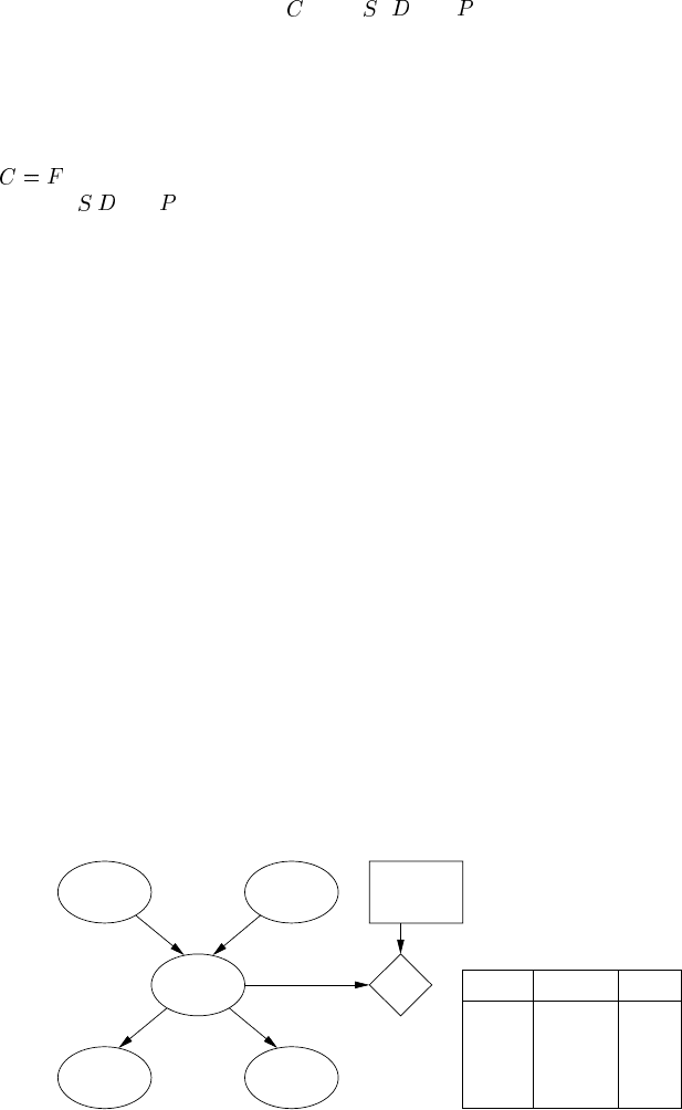
Y
N
−30
0
N
Y
−250
−50
Treatment
U
Cancer
Pollution
Cancer
Smoker
Dyspnoea
XRay
Treatment
U
F
F
T
T
FIGURE 10.1
A decision network for the cancer example.
© 2004 by Chapman & Hall/CRC Press LLC
This whole approach, however, is ad hoc. We are relying on an intuitive (or, at any
rate, unexplicated) judgment about what probability of cancer is worth acting upon.
What we really want is to decide for or against treatment based upon a considera-
tion of the expected value of treatment. The obvious solution is to move to decision
networks, where we can work out the expected utility of both observations and treat-
ments. This is exactly the evaluation of “test-act” combinations that we looked at in
4.4, involving the value of information.
Figure 10.1 shows a decision network for the extended treatment problem. The
effect of different observations on the expected utilities for
are shown in
Table 10.3. We only consider the observations that can increase the belief in cancer
and hence may change the treatment decision. We can see that evidence about any
single node or pair of nodes will not change the decision, because in all cases the
expected utility for not treating remains greater than the expected utility for treating
the patient. However, once we consider the combinations of three evidence nodes,
the decision can change when X-Ray = pos.
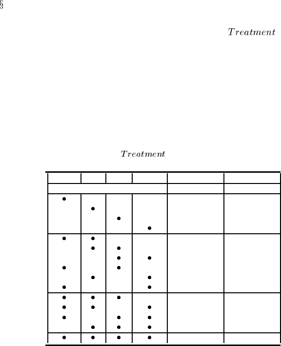
TABLE 10.3
Expected utilities for
in the extended lung cancer
problem (highest expected utility in bold)
X=pos S=T D=T P=high EU(Treat=Y) EU(Treat=N)
No evidence -30.23 -2.908
-31.01 -12.57
-30.64 -8.00
-30.50 -6.22
-30.58 -7.25
-32.59 -32.37
-31.34 -16.71
-31.22 -15.19
-32.06 -25.73
-31.00 -12.50
-32.37 -29.62
-34.88 -60.94
-33.83 -47.87
-34.51 -56.38
-32.05 -25.59
-36.78 -84.78
The work we have done thus far is insufficient, however. While we have now
taken into account the expected utilities of treatment and no treatment, we have not
taken into account the costs of the various observations and tests. This cost may be
purely monetary; more generally, it may combine monetary costs with non-financial
burdens, such as inconvenience, trauma or intrusiveness, as well as some probability
of additional adverse medical outcomes, such as infections caused by examinations
or biopsies.
© 2004 by Chapman & Hall/CRC Press LLC