Jones M., Fleming S.A. Organic Chemistry

Подождите немного. Документ загружается.

1.4 Resonance Forms 29

WORKED PROBLEM 1.18 Add dots for the electron pairs and write resonance

forms for the following structures:

(a)

*(b)

(c)

(d)

(e)

–

CC CC

–

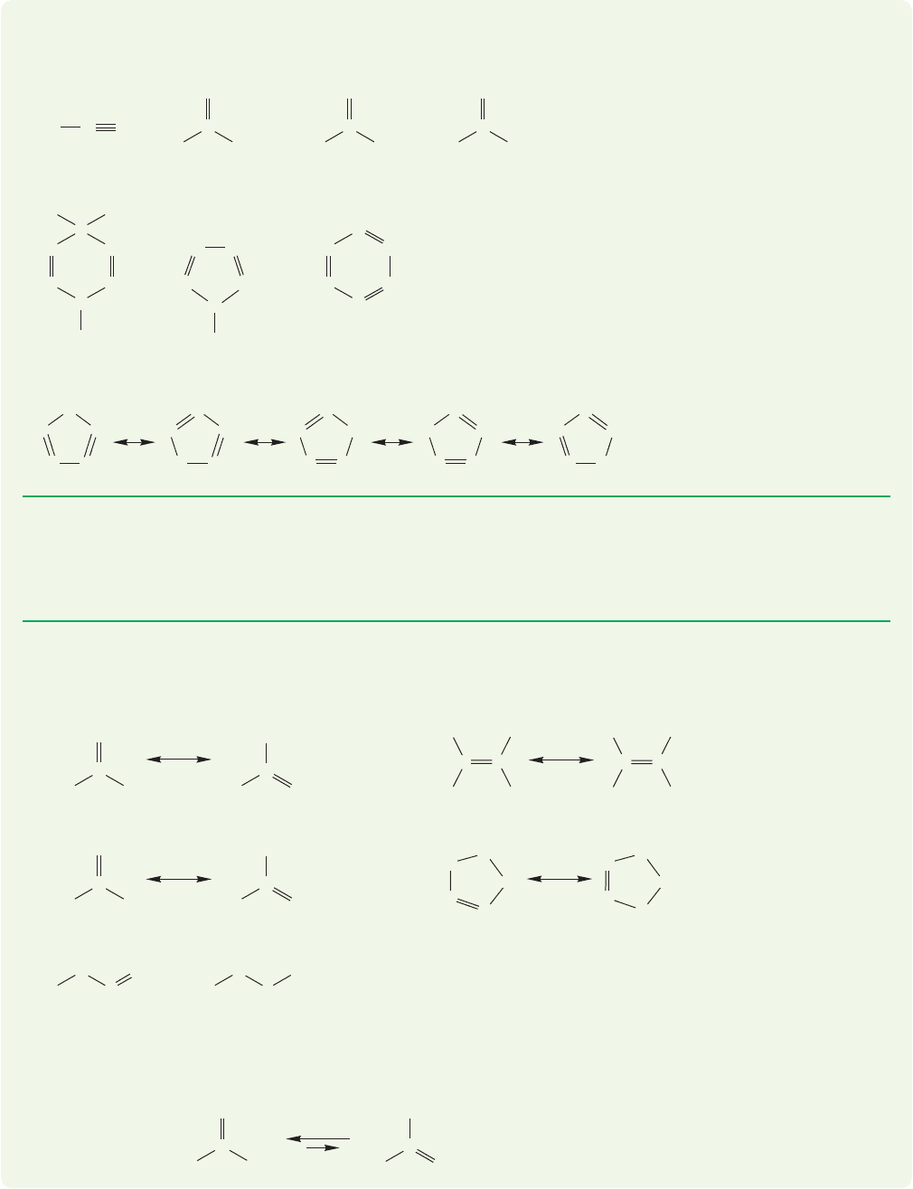
ANSWER (b) These two are not resonance forms because atoms have been moved,

not just electrons. These two molecules are in equilibrium. Molecules related

through the change of position of a single hydrogen are called tautomers.

(a) (b) (c) (d)

(e) *(f) (g)

–

C OCH

–

CHHC

–

CHHC

ANSWER (f)

PROBLEM 1.19 Write Lewis structures and resonance forms for the following

compounds. If you have problems visualizing the structure of some of these mol-

ecules, see the inside front cover of this book.

(a) HONO

(b)



OSO

OH (c) CH

COO



WORKED PROBLEM 1.20 Which of the following pairs of structures are not reso-

nance forms of each other? Why not? You may have to add dots to make good

Lewis structures first.

–

––

–

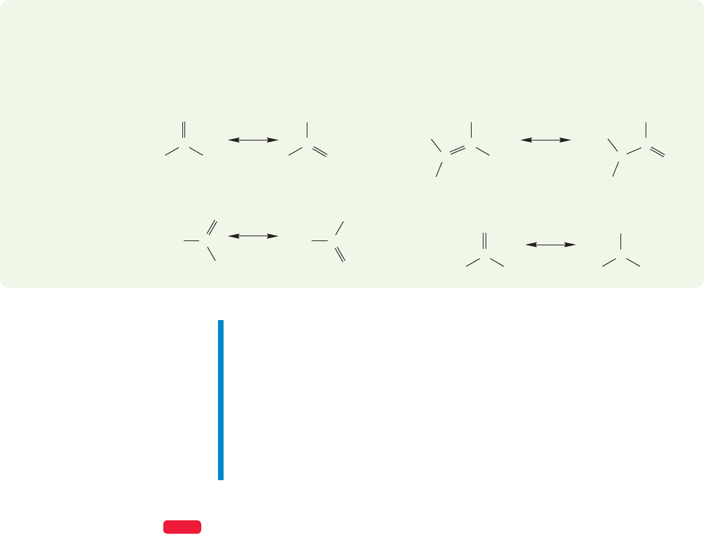
PROBLEM 1.21 In the following pairs of resonance forms, assign weighting factors.

In each case, indicate which form you think is more important,and therefore con-

tributes more to the structure. You may have to add dots to make good Lewis

structures first. Hint: Carbocations are stabilized by substitution.

30 CHAPTER 1 Atoms and Molecules; Orbitals and Bonding

(a)

(b)

(c)

(d)

–

Summary

1. Many molecules are incompletely represented by just one Lewis structure. For

these molecules, resonance structures will provide a more accurate description.

2. Resonance forms are different electronic representations of the same molecule.

3. Resonance forms are not species in equilibrium—molecules do not oscillate back

and forth between resonance forms. The more accurate structure of the

molecule—called the resonance hybrid—is the weighted average of all forms.

4. Some resonance forms contribute more than others to the resonance hybrid.

1.5 Hydrogen (H

): Molecular Orbitals

In the first part of this chapter, we examined atomic structure and atomic orbitals

and began a study of the collections of atoms called molecules. Now we will enlarge

the discussion to include molecular orbitals, the regions of space occupied by elec-

trons in molecules. Covalent bonding between atoms involves the sharing of

electrons.This sharing takes place through overlap of an atomic orbital with anoth-

er atomic orbital or with a molecular orbital.

Chemistry is largely the study of the structure and reactivity of molecules. A cen-

tury ago, when chemistry was a young science,there seemed to be little time to worry

too much about the “how and why” of the science; there was too much discovering

going on, too much information to be collected.

Here is what Friedrich Wöhler (1800–1882), a great early unifier of organic

chemistry, had to say on the subject: “Organic chemistry just now is enough to drive

one mad. It gives one the impression of a primeval, tropical forest full of the most

remarkable things, a monstrous and boundless thicket, with no way of escape, into

which one may well dread to enter.” Nowadays, no longer is some metaphoric vast

jungle being explored by brute force; chemists are now thoughtfully aiming more

and more at new discoveries. The more we understand, and the better our models

of Nature are, the more likely it is that the current transformation from trial-and-

error methods to intellectually driven efforts will be successful.

Directed progress in chemistry depends on understanding how molecules react

and on the application of that understanding in creative ways. These days, the idea

WEB 3D

0 0.50

1.00

Distance between two hydrogens ( )

Energy

1.50 2.502.00 3.00

Energy of

two separated

H atoms

(a)

0.25 Å

Hydrogens

too close



H H

(c)

1 Å

Too far apart

H H

(d)

2 Å

Much too

far apart

molecule

H H

(b)

0.74 Å

Optimum

distance in

the hydrogen

molecule

H H

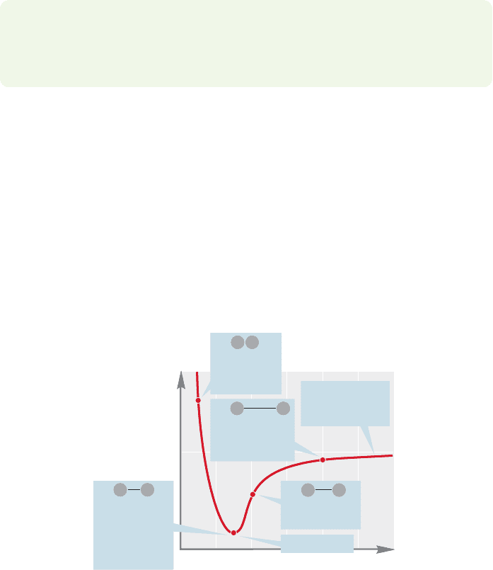
FIGURE 1.36 A plot of the energy for

the hydrogen molecule (H

) as a

function of the distance between the

two hydrogen nuclei.The point of

minimum energy corresponds to the

equilibrium internuclear separation,

the bond distance.

that both the structures of molecules and the reactions they undergo can be under-

stood by examining the shapes and interactions of atomic and molecular orbitals has

gained widespread acceptance in the chemical community, and an important branch

of theoretical chemistry embraces these ideas. Although the study of molecular

orbitals can be approached in a highly mathematical way, we will not follow that

path. One of the great benefits of our nonmathematical approach is that it can be

appreciated quite readily by nonmathematicians! We’ll find that even a very “low

level,” highly qualitative molecular orbital theory can provide striking insights into

structure and reactivity.

In Section 1.3, we constructed Lewis dot structures for molecules. Our next task

is to elaborate on this theme to produce better pictures of the bonds that hold atoms

together in molecules.We’ll need to consider how electrons act to bind nuclei togeth-

er, and we’ll take as our initial example hydrogen (H

),the second simplest molecule.

PROBLEM 1.22 What is the simplest molecule? If H

is the second simplest mol-

ecule, the answer to this question must be “H

minus something.” What might

the “something” be? The answer will appear farther along in the text, so think

about this question for a while now.

We start with two hydrogen atoms,each consisting of a single proton,the nucle-

us, surrounded by an electron in the spherically symmetrical 1s orbital. In principle,

the situation is this simple only as long as the two hydrogen atoms are infinitely far

apart. As soon as they come closer than this infinite distance, they begin to “feel”

each other. Remember: Wave functions do not vanish as the distance from the nucle-

us increases (Fig.1.6). In practice, we can ignore the influence of one hydrogen atom

on the other until they come quite close together, but as soon as they do, the ener-

gy of the system changes greatly. As one hydrogen atom approaches the other, the

energy of the two-atom system decreases until the two hydrogen atoms are 0.74

angstrom (Å, where 1 Å  10

8

cm) apart (Fig. 1.36). From this point the energy

of the system rises sharply, asymptotically approaching infinity as the distance

between the atoms approaches zero.

1.5 Hydrogen (H

): Molecular Orbitals 31

In the hydrogen molecule, two 1s electrons serve to bind the two nuclei togeth-

er. The system is more stable than two separated hydrogen atoms. In the mol-

ecule, the two negatively charged electrons attract both nuclei and hold them

together. When the atoms approach too closely, the positively charged nuclei begin

to repel each other, and the energy goes up sharply.

We begin our mathematical description of bonding by combining the two 1s

atomic orbitals (symbol ψ) of the two hydrogen atoms to produce two new molec-

ular orbitals.The first molecular orbital we will consider is called the bonding molec-

ular orbital. Its symbol is (this Greek letter is

pronounced “fy”). We will use as a shorter notation

for the bonding molecular orbital in this discussion.

Wave function mathematically represents the

bonding molecular orbital and results from a simple

addition of the two atomic orbitals. It can be written as

This bonding molecular orbital is

drawn in Figure 1.37, which shows that looks much like what one would expect

from a simple addition of two spherical 1s orbitals.

Many people use the Greek ψ for both atomic orbitals and molecular

orbitals, but we will use for molecular orbitals. Be careful in your other read-

ing, though, because you will encounter situations in which ψ is used for all

orbitals and even cases where is used for atomic orbitals and ψ for molecular

orbitals!

Because the bonding orbital is concentrated between the two nuclei (Fig.

1.37), two electrons in it can interact strongly with both nuclei. This attraction

explains why the molecular orbital in which the electron density is highest

between the nuclei, is strongly bonding.

Quantum mechanics tells us an important principle: The number of wave func-

tions (orbitals) resulting from the mixing process must equal the number of wave

functions (orbitals) going into the calculation. Because we started by mixing two

hydrogen atomic orbitals, there must be another molecular orbital that is formed.

It is called an antibonding molecular orbital, or (Fig. 1.38), and

results from a subtraction of one atomic orbital from the other to give

Electrons can occupy both bonding and antibonding molecular orbitals.An elec-

tron in a bonding orbital acts to hold the two nuclei together. As the name “anti-

bonding” suggests, an electron in an antibonding orbital does just the opposite—it

contributes to the dissociation of the two nuclei.

There is a third kind of molecular orbital; one in which an electron is neutral in

its effect on the two nuclei. Such an orbital is called a nonbonding orbital. We will

see some nonbonding orbitals when we come to molecules larger than H

By comparing Figures 1.37 and 1.38 you can see that in the antibonding molec-

ular orbital there is a nodal plane between the two hydrogen nuclei. Recall that

a node is a region in which the sign of the wave function is zero. As we pass from

a region where the sign of the wave function is positive to a region in which it is

negative, the sign of must go through zero. As noted earlier, the square of the

wave function corresponds to the electron density, and if is equal to zero, then£

ψ1H

, 1s2 - ψ1H

, 1s2 =£

antibonding

=£

antibonding

ψ1H

, 1s2 + ψ1H

, 1s2 =£

bonding

=£

bonding

32 CHAPTER 1 Atoms and Molecules; Orbitals and Bonding

ψ(H

) = ψ(H

, 1s) ψ(H

) = ψ(H

, 1s) Φ

) = ψ(H

) + ψ(H

)

FIGURE 1.37 The bonding molecular

orbital ( ) of H

.£

ψ(H

) = ψ(H

, 1s) ψ(H

) = ψ(H

, 1s) Φ

) = ψ(H

) – ψ(H

)

Nodal plane

–

FIGURE 1.38 The antibonding

molecular orbital of .1£

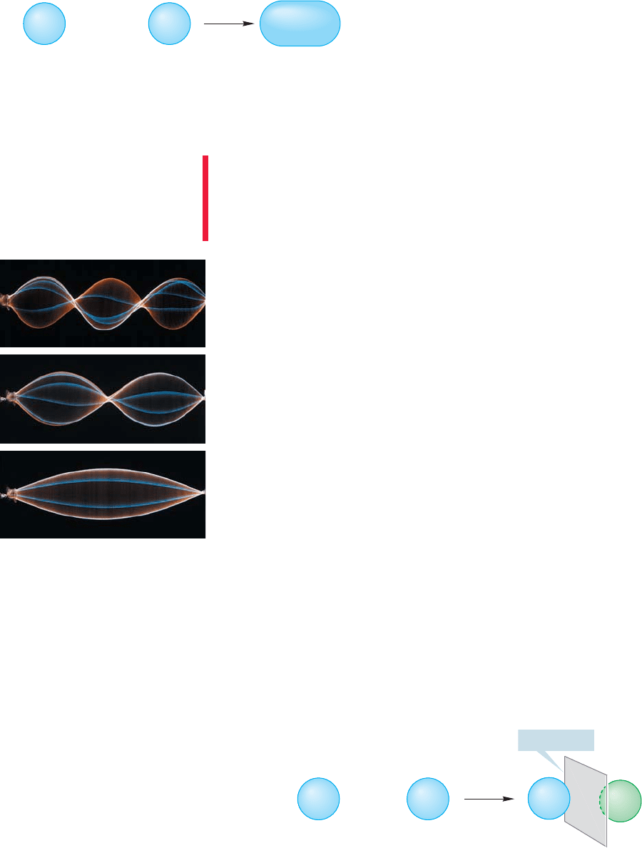
CONVENTION ALERT

Molecular orbitals increase in energy

as the number of nodes increase.

A good analogy is the energy required

to increase the number of nodes in a

jump rope.This photo shows a rope

with zero nodes in the bottom

picture. A rope with one node

requires more energy to generate, and

a rope with two nodes even more.

1.5 Hydrogen (H

): Molecular Orbitals 33

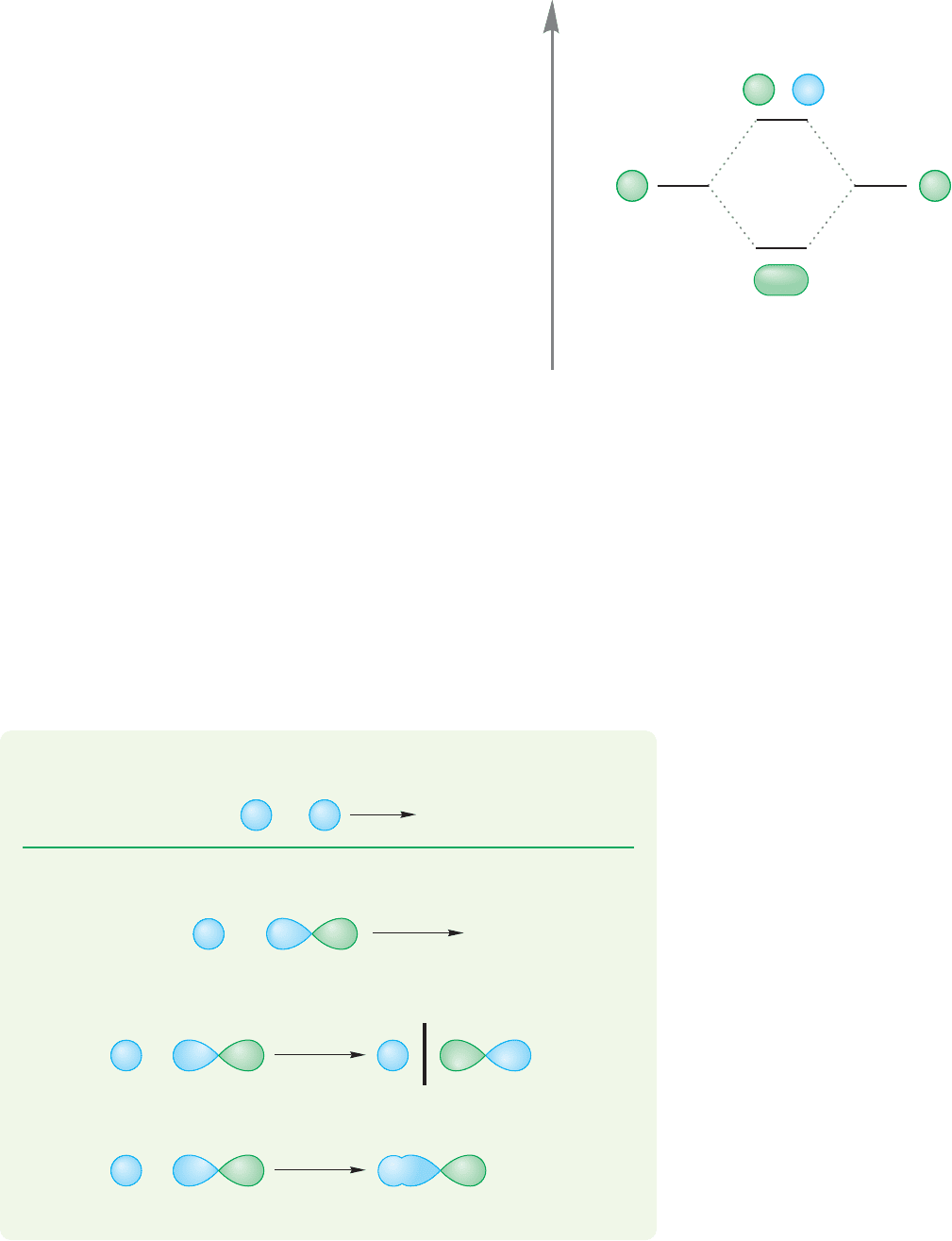
FIGURE 1.39 An orbital interaction

diagram—a graphical representation

of the combination of two atomic 1s

orbitals to form a new bonding and

antibonding pair of molecular

orbitals, and £

.£

is also zero. Therefore the probability of finding an electron

at a node must be zero as well. Accordingly, when a pair of elec-

trons occupies the antibonding molecular orbital of Figure 1.38,

the two nuclei are poorly shielded from each other, and electro-

static repulsion forces the two positively charged nuclei apart.

In summary, the combination of two hydrogen 1s atomic

orbitals yields two new, molecular orbitals, and This

idea seems intuitively reasonable. There are, after all, only two

ways in which two 1s atomic orbitals can be combined to con-

struct two new molecular orbitals. The signs of the wave func-

tions can be either the same, as in the bonding orbital or

opposite, as in the antibonding orbital One common anal-

ogy for this phenomenon is the jump rope, which has wavelike

properties. If we start with a jump rope that has an amplitude

of 3 meters and we add an in-phase wave of the same ampli-

tude, then the result will be a jump rope that has an amplitude

of 6 meters. If,however, we start with the original amplitude and we subtract a wave

(or add an out-of-phase wave) of the same amplitude, then we get a zero amplitude

wave. Subtracting the waves cancels them out.

Figure 1.39 shows a very simple and most useful graphic device for summing up

the energy comparison between atomic orbitals and the molecular orbitals formed

from mixing the orbitals. The graph is called an orbital interaction diagram, or an

interaction diagram for short.The atomic orbitals (ψ) going into the calculation are

shown at the left and right sides of the figure.For molecular hydrogen,these orbitals

are the two equivalent hydrogen 1s atomic orbitals, which must be of the same

energy. They combine in a constructive, bonding way (1s  1s) to give the lower-

energy and in a destructive, antibonding way (1s  1s) to give the higher-

energy Constructive combination for wave functions means that they are

in-phase with each other. Destructive combination means that they are out-of-phase.

PROBLEM 1.23 Sketch the molecular orbitals produced through the interaction of

two carbon 2s atomic orbitals.

WORKED PROBLEM 1.24 Sketch the orbitals produced through the interaction of

a carbon 2s atomic orbital overlapping end-on with a carbon 2p atomic orbital.

ANSWER The two atomic orbitals can interact in a bonding way (2s  2p) or in

an antibonding way (2s  2p):

2s 2p

Antibonding orbital—note

the new node (bar)

Bonding orbital

–

2s 2p

–

.£

= ψ(H

, 1s) – ψ(H

, 1s)

= ψ(H

, 1s) + ψ(H

, 1s)

ψ(H

, 1s) ψ(H

, 1s)

Energy

= ψ(H

, 1s) – ψ(H

, 1s)

= ψ(H

, 1s) + ψ(H

, 1s)

ψ(H

, 1s

) ψ(H

, 1s

)

Stabilization

34 CHAPTER 1 Atoms and Molecules; Orbitals and Bonding

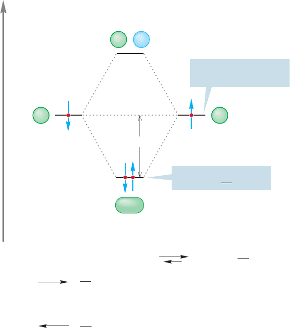
FIGURE 1.40 The electronic

occupancy for the molecule H

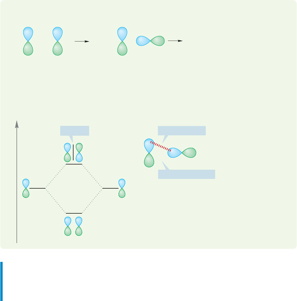
FIGURE 1.41 Two examples of

noninteracting (orthogonal) orbitals.

Note from Figure 1.39 that the orbital interaction diagram is con-

structed without reference to electrons. Only after the diagram has been

constructed do we have to worry about electrons. But now let’s count

them up and put them in the available molecular orbitals. In the con-

struction of H

, each hydrogen atom brings one electron. In

Figure 1.40, these electrons are placed in the appropriate 1s

orbitals ψ and ψ The spin direction of the elec-

trons is shown as paired, but we could also show them as

parallel. In the H

molecule, we put the two electrons into

the lower-energy The electrons must be paired,because

they are in the same orbital and their spin quantum numbers

must be different.The Pauli principle made this point earlier (p. 8).

The antibonding molecular orbital is empty because we are

dealing with only two electrons and they are both accommodated in the

bonding molecular orbital.

So far we have dealt only with mixing one atomic orbital with another atomic

orbital. But it is also possible to mix a molecular orbital with another molecular

orbital or an atomic orbital with a molecular orbital.Not all combinations of orbitals

are productive. If two orbitals approach each other in such a way that the new bond-

ing interactions are exactly balanced by antibonding interactions, there is no net inter-

action between the two and no bond would form.Such orbitals are called orthogonal

orbitals, orbitals that do not mix.Therefore,the way in which orbitals approach each

other in space—how the lobes overlap—is critically important. Figure 1.41 shows

two cases of atomic orbitals that are orthogonal to each other. As the orbitals

approach each other, the number of bonding overlaps (shown with red dashed line)

and antibonding overlaps are the same. The result is no net bonding. In each case,

as the orbitals are brought together the bonding interactions (blue–blue starting to

overlap) are exactly canceled by the antibonding interactions (blue–green starting

to overlap).

Here are some “rules” for orbital construction:

1. The number of orbitals produced must equal the number of orbitals you begin with.

If you start with n orbitals, you must produce n new orbitals. Here is a way to check

your work as you proceed.

2. Keep the process as simple as you can. Use what you know already, and combine

orbitals in as symmetrical a fashion as you can.

3. The closer in energy two orbitals are, the more strongly they interact. At this prim-

itive (but useful) level of theory, you need mix only the pairs of orbitals closest in

energy to each other.

4. When two orbitals interact in a bonding way (wave functions for the two orbitals

have same sign), the energy of the resulting orbital is lowered; when they interact

in an antibonding way (wave functions have different signs), the energy of the

resulting orbital is raised.

5. When two orbitals interact, the only options for mixing are adding (in-phase mixing)

or subtracting (out-of-phase mixing). When three orbitals interact we will have

1£

2.1H

There can be no denying that the concept of an empty antibonding orbital is slippery! It makes physicists

very uneasy, for example. Chemists see the empty orbital of Figures 1.39 and 1.40 as “the place the next elec-

tron would go.”

Antibonding

Bonding

Antibonding

Bonding

1.5 Hydrogen (H

): Molecular Orbitals 35

three ways to mix the orbitals. With four orbitals there are four combinations

possible, and so on.

6. To put new orbitals in order according to their energy, count the nodes. For a given

molecule, the more nodes in an orbital, the higher it is in energy.

There is a connection between stability and energy. The lower the energy of an

orbital, the greater the stability of an electron in it. A consequence of this stability is

that the strongest bonds in molecules are formed by electrons occupying the lowest-

energy molecular orbitals.Throughout this chapter we will be taking note of what fac-

tors lead to low-energy molecular orbitals and thus to strong bonding between atoms.

WORKED PROBLEM 1.25 Contrast the interactions between two 2p orbitals

approaching in the two different ways shown below.

ANSWER (a) A pair of 2p atomic orbitals aligned parallel to each other interacting

side by side produces two new molecular orbitals, one bonding (2p  2p) and one

antibonding (2p  2p). (b) The orbitals aligned perpendicular to each other produce

no molecular orbitals because there is no net bonding or antibonding.The two exact-

ly cancel, producing no net interaction. In this case, the two orbitals are orthogonal.

Perpendicular

–

Parallel

(a) (b)

–

(a)

Energy

2p 2p

2p2p

2p 2p

Antibonding orbital

Bonding orbital

New node

–

Bonding interaction

There is no net interaction

here as the bonding and

antibonding interactions

(overlaps) exactly cancel

Antibonding interaction

(b)

Summary

Overlap of two atomic orbitals produces two new molecular orbitals, one bond-

ing and the other antibonding.Two electrons can be accommodated in the lower-

energy bonding molecular orbital. In this way, two atoms (or groups of atoms)

can be bound through the sharing of electrons in a covalent bond.

36 CHAPTER 1 Atoms and Molecules; Orbitals and Bonding

104 kcal/mol

Energy of two separate

hydrogen atoms, 2 H

Energy of one hydrogen

molecule, H

Two separate hydrogen atoms molecular H H, H

H H

ΔH° = –104 kcal/mol

This reaction is exothermic by 104 kcal/mol

H H

ΔH° = +104 kcal/mol

This reaction is endothermic by 104 kcal/mol

ψ(H

, 1s

) ψ(H

, 1s

)

Energy

FIGURE 1.42 Molecular hydrogen

) is more stable than two isolated

hydrogen atoms by 104 kcal/mol.

1.6 Bond Strength

In Figure 1.40, the energy of the electrons in the two atomic orbitals is greater than

their energy in the bonding molecular orbital As noted earlier, lower energy

means greater stability, but just how much energy is the stabilization apparent in

Figure 1.40 worth? The difference between the energies of the two electrons in

and the energies of the two separate electrons in atomic 1s orbitals is 104 kcal/mol.

This amount of energy is very large, and consequently the H

molecule is held

together (bound) by a substantial amount of energy; this amount of energy is

released into the environment if H

molecules are formed from separated hydrogen

atoms. It would require the application of exactly this amount of energy to gener-

ate two hydrogen atoms from a molecule of H

. The 104 kcal/mol represents the

stabilization of two electrons in (Fig. 1.42).

Actually, if we could measure it, the temperature would rise ever so slightly as

two hydrogen atoms combined to make a hydrogen molecule because 104 kcal/mol

would be released as heat energy into the vessel.The environment in the vessel would

warm up as the process proceeded.A reaction that liberates heat,one where the prod-

ucts are more stable than the starting materials, is called an exothermic reaction.

The opposite situation, in which the products are less stable than the starting ma-

terial, requires the application of heat and is called an endothermic reaction.

The enthalpy change of any chemical reaction is estimated as the differ-

ence between the total bond energy of the products and the total bond energy of

(≤H°)

1.6 Bond Strength 37

the reactants.The value of for a reaction between hydrogen atoms to give H

is 104 kcal/mol.

The sometimes troublesome sign convention shows for an exothermic

reaction as a negative quantity. For an endothermic reaction, is positive. For

example,

If A  B C then the reaction is exothermic

If A  B C then the reaction is endothermic

In Figure 1.42

is an exothermic reaction

From this we can also know that the reverse reaction

is an endothermic reaction

Figure 1.43 is a graph that plots the energy of reactants and products in a

chemical reaction against a variable known either as the reaction progress or the

reaction coordinate. A reaction coordinate monitors a change or changes taking

place as the reaction proceeds. These changes may be distance between atoms,

angles between bonds, or a combination of relationships that result from the

movement of atoms. For example, in the reaction a suitable

reaction coordinate might be the distance between the two hydrogen atoms. It is

a fair approximation at this point to take this “reaction coordinate” as indicative

of the progress of the overall reaction, and for that reason we will use the term

reaction progress from now on.

A reaction progress graph can be read either left to right or right to left.Reading

Figure 1.43 left to right tells us that the energy of the product is lower than the ener-

gy of the reactants, and so the graph shows the release of energy, in this case,

104 kcal/mol, as H

is formed in an exothermic reaction. If we read the graph from

right to left,we see the endothermic formation of two hydrogen atoms from the H

molecule.

This amount of energy that must be added to break the H

bond to produce two

hydrogen atoms, 104 kcal/mol, is called the bond dissociation energy (BDE). It is

the amount of energy that must be applied for homolytic bond cleavage.The high-

er the BDE, the more difficult it is to break the bond. A bond can break in either

of two ways (Fig. 1.44). In the homolytic cleavage, one electron from the bond goes

with one atom and the other electron of the bond goes with the other atom. This

kind of bond cleavage gives neutral species.The other option for bond breaking has

both electrons from the bond go to the same atom creating an anion–cation pair.

This process is called heterolytic bond cleavage. Normally, heterolytic cleavage is

not the path followed because it usually costs more energy to develop separated

charges than to make neutral species.

+ H

¢H ° =+104 kcal>mol,H

+ H

¢H ° =-104 kcal>mol,H

+ H

¢H ° =+x kcal>mol,

¢H ° =-x kcal>mol,

¢H °

104 kcal/mol

H H

Reaction progress

(reaction coordinate)

Energy

FIGURE 1.43 Another schematic

picture of the formation of molecular

hydrogen from two hydrogen atoms.

CONVENTION ALERT

Two versions of heterolytic bond

cleavage for the molecule

ions are formed

Homolytic bond cleavage

for the molecule X

neutral species are formed

–

FIGURE 1.44 In one kind of bond

cleavage, the pair of binding electrons

is split evenly between the atoms,

giving a pair of neutral species.This

lower-energy process is called

homolytic cleavage. Heterolytic

cleavage produces a pair of ions.

38 CHAPTER 1 Atoms and Molecules; Orbitals and Bonding

Notice the difference in the red curved arrows in the two parts of Figure 1.44.The

curved arrow showing electron movement in the heterolytic cleavage has the stan-

dard double-barbed arrows, representing the movement of two electrons to the same

atom. The homolytic cleavage pathway uses single-barbed or “fishhook” arrows rep-

resenting the movement of one electron to each atom.

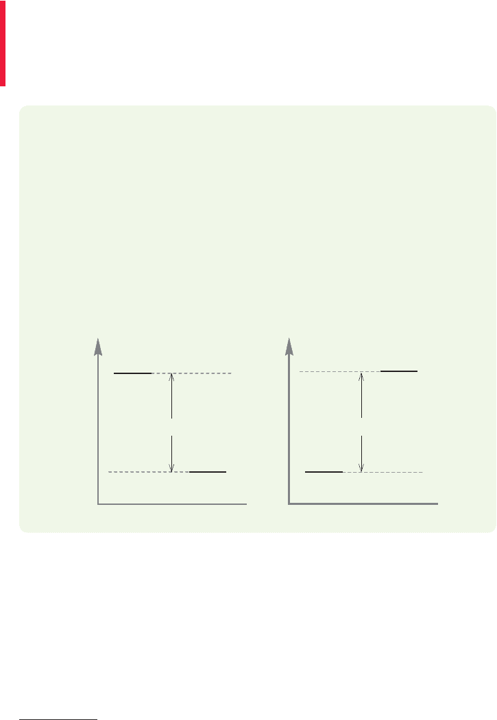
WORKED PROBLEM 1.26 Sketch the profile of an endothermic reaction. See Figure

1.43 for the sketch of an exothermic reaction.

ANSWER Aha! A trick question. If you have written an exothermic reaction, you

have already written an endothermic reaction as well. You need only read your

answer backward. We are psychological prisoners of our tendency to read from

left to right. Nature has no such hangups! The formation of molecular hydrogen

from two hydrogen atoms (Fig. 1.43, left to right) is exothermic (104 kcal/mol of

energy is given off as heat), and the formation of two hydrogen atoms from a sin-

gle hydrogen molecule is endothermic by the same amount (104 kcal/mol of heat

energy must be applied).

In practice,a reaction that requires about 15–20 kcal/mol of thermal energy pro-

ceeds quite reasonably at room temperature, about 25 °C. It is important to begin to

develop a feeling for which bonds are strong and which are weak, to start to build

up a knowledge of approximate bond strengths.

The bond in the hydrogen mol-

ecule is a strong one. As we continue our discussion of structure, we’ll make a point

of noting bond energies as we go along. Unfortunately, there is no way to acquire

this knowledge except by learning some bond strengths. Fortunately, there are not

too many numbers to remember. Table 1.9 gives a few important bond dissociation

Energy

Reaction progress

Exothermic formation

of H

from 2 H

Endothermic formation

of 2 H from H

2 H

Energy

2 H

104 kcal/mol

To describe a bond as strong or weak is an arbitrary function of human experience. A bond that requires

100 kcal/mol to break is “strong”in a world where room temperature supplies much less thermal energy.It would

not be strong on the sunlit side of Mercury (where it’s hot: the average temperature is about 377 °C,or 710 °F).

Similarly, if you were a life form that evolved on Pluto (where it’s cold: the average temperature is about 220 °C,

or 361 °F), you would regard as strong all sorts of “weak” (on Earth) interactions, and your study of chem-

istry would be very different indeed. One area of research in organic chemistry focuses on extremely unstable

molecules held together by weak bonds. The idea is that by understanding extreme forms of weak bonding

we can learn more about the forces that hold together more conventional molecules. Chemists who work in

this area deliberately devise conditions under which species that are normally most unstable can be isolated.

They create very low temperature “worlds” in which other reactive (predatory) molecules are absent. In such

a world, exotic species may be stable, as they are insulated from both the ravages of heat (thermodynamic sta-

bility) and the predations of other molecules (kinetic stability).

CONVENTION ALERT