Jacques I. Mathematics for Economics and Business
Подождите немного. Документ загружается.

Hence an increase in I* leads to an increase in C. If
a =
1
/
2 then
==1
Change in C is
1 × 2 = 2
2 (a) Substitute C, I, G, X and M into the Y equation to get
Y = aY + b + I* + G* + X * − (mY + M *)
Collecting like terms gives
(1 − a + m)Y = b + I * + G* + X* − M*
so
Y =
(b) =
=−
Now a < 1 and m > 0, so 1 − a + m > 0. The
autonomous export multiplier is positive, so
an increase in X* leads to an increase in Y. The
marginal propensity to import multiplier is
negative. To see this note from part (a) that
∂Y/∂m can be written as
−
and Y
> 0 and 1 − a + m > 0.
(c) Y =
= 2100
==
and
∆X* = 10
so
∆Y =×10 =
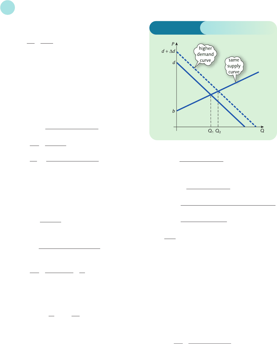
3 If d increases by a small amount then the intercept
increases and the demand curve shifts upwards slightly.
Figure S5.2 shows that the effect is to increase the
equilibrium quantity from Q
1
to Q
2
, confirming that
∂Q/∂d > 0.
4 (a) Substituting equations (3) and (4) into (2) gives
C = a(Y − T *) + b = aY − aT* + b (7)
Substituting (5), (6) and (7) into (1) gives
Y = aY − aT * + b + I * + G*
100
3
10
3
10
3
1
1 − 0.8 + 0.1
∂Y
∂X*
120 + 100 + 300 + 150 − 40
1 − 0.8 + 0.1
Y
1 − a + m
b + I* + G* + X* − M*
(1 − a + m)
2
∂Y
∂m
1
1 − a + m
∂Y
∂X*
b + I* + G* + X* − M *
1 − a + m
1
/2
1 −
1
/2
∂C
∂I*
so that
Y =
Finally, from (7), we see that
C = a − aT* + b
=
=
(b) > 0; C increases. (c) 1520; rise of 18.
5(1)From the relations
C = aY
d
+ b
Y
d
= Y − T
T = tY + T*
we see that
C = a(Y − tY − T *) + b
Similarly,
M = m(Y − tY − T *) + M*
Substitute these together with I, G and X into the Y
equation to get the desired result.
(2) (a) =
Numerator is negative because m < a.
Denominator can be written as
(1 − a) + at + m(1 − t)
which represents the sum of three positive
numbers, so is positive. Hence the autonomous
taxation multiplier is negative.
m − a
1 − a + at + m − mt
∂Y
∂T*
a
1 − a
aI* + aG* − aT* + b
1 − a
a(−aT* + b + I* + G*) + (1 − a)(−aT* + b)
1 − a
D
F
−aT* + b + I* + G*
1 − a
A
C
−aT* + b + I* + G*
1 − a
Solutions to Problems
640
Figure S5.2
MFE_Z02.qxd 16/12/2005 10:51 Page 640
(b) =>0
(3) (a) 1000; (b) ∆Y = 20; (c) ∆T* = 33
1
/3.
6 From text, equilibrium quantity is
Substituting this into either the supply or demand
equation gives the desired result.
=>0, =>0
=− <0, =>0
where the quotient rule is used to obtain ∂P/∂a
and ∂P/∂c. An increase in a, b or d leads to an
increase in P, whereas an increase in c leads to a
decrease in P.
7(1)Substituting second and third equations into first
gives
Y = aY + b + cr + d
so that
(1 − a)Y − cr = b + d (1)
(2) Substituting first and second equations into third
gives
k
1
Y + k
2
r + k
3
= M *
S
so that
k
1
Y + k
2
r = M*
S
− k
3
(2)
(3) (a) Working out c × (2) + k
2
× (1) eliminates r to
give
ck
1
Y + k
2
(1 − a)Y
= c(M *
S
− k
3
) + k
2
(b + d)
Dividing both sides by ck
1
+ k
2
(1 − a) gives
result.
(b) , which is positive because the top
and bottom of this fraction are both negative.
Section 5.4
1 f
x
= 2x, f
y
= 6 − 6y, f
xx
= 2, f
yy
=−6, f
xy
= 0.
Step 1
At a stationary point
2x = 0
6 − 6y = 0
which shows that there is just one stationary point
at (0, 1).
c
(1 − a)k
2
+ ck
1
a
a + c
∂P
∂d
a(d − b)
(a + c)
2
∂P
∂c
c
a + c
∂P
∂b
c(d − b)
(a + c)
2
∂P
∂a
d− b
a + c
1
1 − a + at + m − mt
∂Y
∂G*
Step 2
f
xx
f
yy
− f
2
xy
= 2(−6) − 0
2
=−12 < 0
so it is a saddle point.
2 Total revenue from the sale of G1 is
TR
1
= P
1
Q
1
= (50 − Q
1
)Q
1
= 50Q
1
− Q
1
2
Total revenue from the sale of G2 is
TR
2
= P
2
Q
2
= (95 − 3Q
2
)Q
2
= 95Q
2
− 3Q
2
2
Total revenue from the sale of both goods is
TR = TR
1
+ TR
2
= 50Q
1
− Q
1
2
+ 95Q
2
− 3Q
2
2
Profit is
π=TR − TC
= (50Q
1
− Q
1
2
+ 95Q
2
− 3Q
2
2
) − (Q
1
2
+ 3Q
1
Q
2
+ Q
2
2
)
= 50Q
1
− 2Q
1
2
+ 95Q
2
− 4Q
2
2
− 3Q
1
Q
2
Now
= 50 − 4Q
1
− 3Q
2
,
= 95 − 8Q
2
− 3Q
1
=−4, =−3,
=−8
Step 1
At a stationary point
50 − 4Q
1
− 3Q
2
= 0
95 − 3Q
1
− 8Q
2
= 0
that is,
4Q
1
+ 3Q
2
= 50 (1)
3Q
1
+ 8Q
2
= 95 (2)
Multiply equation (1) by 3, and equation (2) by 4 and
subtract to get
23Q
2
= 230
so Q
2
= 10. Substituting this into either equation (1) or
equation (2) gives Q
1
= 5.
Step 2
This is a maximum because
=−4 < 0, =−8 < 0
and
∂
2
π
∂Q
2
2
∂
2
π
∂Q
1
2
∂
2
π
∂Q
2
2
∂
2
π
∂Q
1
∂Q
2
∂
2
π
∂Q
1
2
∂π
∂Q
2
∂π
∂Q
1
Solutions to Problems
641
MFE_Z02.qxd 16/12/2005 10:51 Page 641

−
2
= (−4)(−8) − (−3)
2
= 23 > 0
Corresponding prices are found by substituting Q
1
= 5
and Q
2
= 10 into the original demand equations to
obtain P
1
= 45 and P
2
= 65.
3 For the domestic market, P
1
= 300 − Q
1
, so
TR
1
= P
1
Q
1
= 300Q
1
− Q
1
2
For the foreign market, P
2
= 200 −
1
/2Q
2
, so
TR
2
= P
2
Q
2
= 200Q
2
−
1
/2Q
2
2
Hence
TR = TR
1
+ TR
2
= 300Q
1
− Q
1
2
+ 200Q
2
−
1
/
2
Q
2
2
We are given that
TC = 5000 + 100(Q
1
+ Q
2
)
= 5000 + 100Q
1
+ 100Q
2
so
π=TR − TC
= (300Q
1
− Q
1
2
+ 200Q
2
−
1
/
2
Q
2
2
) − (5000
+ 100Q
1
+ 100Q
2
)
= 200Q
1
− Q
1
2
+ 100Q
2
−
1
/2Q
2
2
− 5000
Now
= 200 − 2Q
1
, = 100 − 2Q
2
=−2, = 0, =−1
Step 1
At a stationary point
200 − 2Q
1
= 0
100 − Q
2
= 0
which have solution Q
1
= 100, Q
2
= 100.
Step 2
This is a maximum because
=−2 < 0,
=−1 < 0
and
−
2
= (−2)(−1) − 0
2
= 2 > 0
D
F
∂
2
π
∂Q
1
∂Q
2
A
C
D
F
∂
2
π
∂Q
2
2
A
C
D
F
∂
2
π
∂Q
1
2
A
C
∂
2
π
∂Q
2
2
∂
2
π
∂Q
1
2
∂
2
π
∂Q
2
2
∂
2
π
∂Q
2
1
∂Q
2
∂
2
π
∂Q
1
2
∂π
∂Q
2
∂π
∂Q
1
D
F
∂
2
π
∂Q
1
∂Q
2
A
C
D
F
∂
2
π
∂Q
2
2
A
C
D
F
∂
2
π
∂Q
1
2
A
C
Substitute Q
1
= 100, Q
2
= 100, into the demand
and profit functions to get P
1
= 200, P
2
= 150 and
π=10 000.
4 (a) Minimum at (1, 1), maximum at (−1, −1), and
saddle points at (1, −1) and (−1, 1).
(b) Minimum at (2, 0), maximum at (0, 0), and saddle
points at (1, 1) and (1, −1).
5 Maximum profit is $1300 when Q
1
= 30 and Q
2
= 10.
6 Maximum profit is $95 when P
1
= 30 and P
2
= 20.
7 Maximum profit is $176 when L = 16 and K = 144.
8 x
1
= 138, x
2
= 500; $16.67 per hour.
9 Q
1
= 19, Q
2
= 4.
10 (a) Minimum at (1, 2).
(b) Maximum at (0, 1).
(c) Saddle point at (2, 2).
11 (a) P
1
= 78, P
2
= 68.
(b) Rotate the box so that the Q
1
axis comes straight
out of the screen. The graph increases steadily as
Q
2
rises from 0 to 2.
Q
1
= 24. Profit in (a) and (b) is 1340 and 1300
respectively.
Section 5.5
1 Step 1
We are given that y = x, so no rearrangement is necessary.
Step 2
Substituting y = x into the objective function
z = 2x
2
− 3xy + 2y + 10
gives
z = 2x
2
− 3x
2
+ 2x + 10
=−x
2
+ 2x + 10
Step 3
At a stationary point
= 0
that is,
−2x + 2 = 0
which has solution x = 1. Differentiating a second time
gives
=−2
confirming that the stationary point is a maximum.
d
2
z
dx
2
dz
dx
Solutions to Problems
642
MFE_Z02.qxd 16/12/2005 10:51 Page 642
The value of z can be found by substituting x = 1 into
z =−2x
2
+ 2x + 10
to get z = 11. Finally, putting x = 1 into the constraint
y = x gives y = 1. The constrained function therefore
has a maximum value of 11 at the point (1, 1).
2 We want to maximize the objective function
U = x
1
x
2
subject to the budgetary constraint
2x
1
+ 10x
2
= 400
Step 1
x
1
= 200 − 5x
2
Step 2
U = 200x
2
− 5x
2
2
Step 3
= 200 − 10x
2
= 0
has solution x
2
= 20.
=−10 < 0
so maximum.
Putting x
2
= 20 into constraint gives x
1
= 100.
U
1
==x
2
= 20
and
U
2
==x
2
= 100
so the ratios of marginal utilities to prices are
==10
and
==10
which are the same.
3 We want to minimize the objective function
TC = 3x
2
1
+ 2x
1
x
2
+ 7x
2
2
subject to the production constraint
x
1
+ x
2
= 40
Step 1
x
1
= 40 − x
2
100
10
U
2
P
2
20
2
U
1
P
1
∂U
∂x
2
∂U
∂x
1
d
2
U
dx
2
2
dU
dx
1
Step 2
TC = 3(40 − x
2
)
2
+ 2(40 − x
2
)x
2
+ 7x
2
2
= 4800 − 160x
2
+ 8x
2
2
Step 3
=−160 + 16x
2
= 0
has solution x
2
= 10.
= 16 > 0
so minimum.
Finally, putting x
2
= 10 into constraint gives x
1
= 30.
4 Maximum value of z is 13, which occurs at (3, 11).
5 27 000.
6 K = 10 and L = 4.
7 K = 6 and L = 4.
8 Maximum profit is $165, which is achieved when K = 81
and L = 9.
9 x
1
= 3, x
2
= 4.
Section 5.6
1 Step 1
g(x, y, λ) = 2x
2
− xy +λ(12 − x − y)
Step 2
= 4x − y −λ=0
=−x −λ=0
= 12 − x − y = 0
that is,
4x − y −λ=0 (1)
−x −λ=0 (2)
x + y = 12 (3)
Multiply equation (2) by 4 and add equation (1), multiply
equation (3) by 4 and subtract from equation (1) to get
−y − 5λ=0 (4)
−5y − λ=−48 (5)
Multiply equation (4) by 5 and subtract equation (5) to
get
−24λ=48 (6)
Equations (6), (5) and (1) can be solved in turn to get
λ=−2, y = 10, x = 2
∂g
∂λ
∂g
∂y
∂g
∂x
d
2
(TC)
dx
2
2
d(TC)
dx
2
Solutions to Problems
643
MFE_Z02.qxd 16/12/2005 10:51 Page 643
so the optimal point has coordinates (2, 10). The
corresponding value of the objective function is
2(2)
2
− 2(10) =−12
2 Maximize
U = 2x
1
x
2
+ 3x
1
subject to
x
1
+ 2x
2
= 83
Step 1
g(x
1
, x
2
, λ) = 2x
1
x
2
+ 3x
1
+λ(83 − x
1
− 2x
2
)
Step 2
= 2x
2
+ 3 −λ=0
= 2x
1
− 2λ=0
= 83 − x
1
− 2x
2
= 0
that is,
2x
2
−λ=−3 (1)
2x
1
− 2λ=0 (2)
x
1
+ 2x
2
= 83 (3)
The easiest way of solving this system is to use
equations (1) and (2) to get
λ=2x
2
+ 3 and λ=x
1
respectively. Hence
x
1
= 2x
2
+ 3
Substituting this into equation (3) gives
4x
2
+ 3 = 83
which has solution x
2
= 20 and so x
1
=λ=43.
The corresponding value of U is
2(43)(20) + 3(43) = 1849
The value of λ is 43, so when income rises by 1 unit,
utility increases by approximately 43 to 1892.
3 Step 1
g(x
1
, x
2
, λ) = x
1
1/2
+ x
2
1/2
+λ(M − P
1
x
1
− P
2
x
2
)
Step 2
= x
1
−1/2
−λP
1
= 0 (1)
= x
2
−1/2
−λP
2
= 0 (2)
= M − P
1
x
1
− P
2
x
2
= 0 (3)
∂g
∂λ
1
2
∂g
∂x
2
1
2
∂g
∂x
1
∂g
∂λ
∂g
∂x
2
∂g
∂x
1
From equations (1) and (2)
λ= and λ=
respectively. Hence
=
that is,
x
1
P
1
2
= x
2
P
2
2
so
x
1
= (4)
Substituting this into equation (3) gives
M −−P
2
x
2
= 0
which rearranges as
x
2
=
Substitute this into equation (4) to get
x
1
=
4 9.
5 There are two wheels per frame, so the constraint is
y = 2x. Maximum profit is $4800 at x = 40, y = 80.
6 Maximum profit is $600 at Q
1
= 10, Q
2
= 5. Lagrange
multiplier is 4, so profit rises to $604 when total cost
increases by 1 unit.
7 40; 2.5.
8 x
1
= and x
2
=
Chapter 6
Section 6.1
1 (a) x
2
; (b) x
4
; (c) x
100
; (d) x
4
; (e) x
19
.
2 (a) x
5
+ c; (b) −+c; (c) x
4/3
+ c;
(d) e
3x
+ c; (e) x + c;
(f) + c; (g) ln x + c.
3 (a) x
2
− x
4
+ c; (b) 2x
5
−+c;
(c) x
3
− x
2
+ 2x + c.
3
2
7
3
5
x
x
2
2
1
3
3
4
1
2x
2
1
5
1
19
1
4
βM
(α+β)P
2
αM
(α+β)P
1
P
2
M
P
1
(P
1
+ P
2
)
P
1
M
P
2
(P
1
+ P
2
)
x
2
P
2
2
P
1
x
2
P
2
2
P
1
2
1
2x
2
1/2
P
2
1
2x
1
1/2
P
1
1
2x
2
1/2
P
2
1
2x
1
1/2
P
1
Solutions to Problems
644
MFE_Z02.qxd 16/12/2005 10:51 Page 644

4 (a) TC =
2dQ = 2Q + c
Fixed costs are 500, so c = 500. Hence
TC = 2Q + 500
Put Q = 40 to get TC = 580.
(b) TR =
(100 − 6Q)dQ
= 100Q − 3Q
2
+ c
Revenue is zero when Q = 0, so c = 0. Hence
TR = 100Q − 3Q
2
P ==
= 100 − 3Q
so demand equation is P = 100 − 3Q.
(c) S =
(0.4 − 0.1Y
−1/2
)dY
= 0.4Y − 0.2Y
1/2
+ c
The condition S = 0 when Y = 100 gives
0 = 0.4(100) − 0.2(100)
1/2
+ c
= 38 + c
so c =−38. Hence
S = 0.4Y − 0.2Y
1/2
− 38
5 (a) x
6
+ c; (b) x
5
+ c; (c) e
10x
+ c; (d) ln x + c;
(e) x
5/2
+ c; (f) x
4
− 3x
2
+ c;
(g) x
3
− 4x
2
+ 3x + c; (h) + bx + c;
(i) x
4
− 2e
−2x
++c.
6 (1) F′(x) = 10(2x + 1)
4
, which is 10 times too big, so
the integral is
(2x + 1)
5
+ c
(2) (a) (3x − 2)
8
+ c; (b) − (2 − 4x)
10
+ c;
(c) (ax + b)
n+1
+ c; (d) ln(7x + 3) + c.
7 (a) TC =+5Q + 20
(b) TC = 6e
0.5Q
+ 4
8 (a) TR = 20Q − Q
2
; P = 20 − Q
(b) TR = 12 Q; P =
12
Q
Q
2
2
1
7
1
a(x + 1)
1
40
1
24
1
10
3
x
7
4
ax
2
2
1
3
1
2
2
5
1
5
100Q − 3Q
2
Q
TR
Q
9 C = 0.6Y + 7, S = 0.4Y − 7
10 (a) 1000L − L
3
(b) 12√L − 0.01L
11 (a) x
2
+ x
7/2
+ c
(b) x
11
+ x
3
; e
5x
+ e
x
+ e
2x
+ c; x
3
− x
2
+ c.
12 (a) x
4
− x
2
+ 2
1/2
x + c
(b) ln x ++c; −e
−x
+ e
−3x
+ c; x − x + x
3/2
+ c
13 +√Y + 3; k = 9.
14 (a) 500Le
−0.02L
; (b) ln(1 + 50Q
2
).
Section 6.2
1 (a)
1
0
x
3
dx = x
4
1
0
= (1)
4
− (0)
4
=
(b)
5
2
(2x − 1)dx = [x
2
− x]
5
2
= (5
2
− 5) − (2
2
− 2) = 18
(c)
4
1
(x
2
− x + 1)dx
= x
3
− x
2
+ x
4
1
= (4)
3
− (4)
2
+ 4 − (1)
3
− (1)
2
+ 1
= 16.5
(d)
1
0
e
x
dx = [e
x
]
1
0
= e
1
− e
0
= e − 1 = 1.718 28...
2 Substitute Q = 8 to get
P = 100 − 8
2
= 36
CS =
8
0
(100 − Q
2
)dQ − 8(36)
= 100Q − Q
3
8
0
− 288
= 100(8) − (8)
3
− 100(0) − (0)
2
− 288
= 341.33
3 In equilibrium, Q
S
= Q
D
= Q, so
P = 50 − 2Q
P = 10 + 2Q
J
L
1
3
G
I
J
L
1
3
G
I
J
L
1
3
G
I
J
L
1
2
1
3
G
I
J
L
1
2
1
3
G
I
J
L
1
2
1
3
G
I
1
4
1
4
1
4
J
L
1
4
G
I
Y
3
2
3
1
3
1
x
1
2
1
4
1
2
1
3
3
2
1
5
1
3
1
11
2
7
1
2
Solutions to Problems
645
MFE_Z02.qxd 16/12/2005 10:51 Page 645
Hence
50 − 2Q = 10 + 2Q
which has solution Q = 10. The demand equation gives
P = 50 − 2(10) = 30
(a) CS =
0
10
(50 − 2Q)dQ − 10(30)
= [50Q − Q
2
]
0
10
− 300
= [50(10) − (10)
2
] − [50(0) − 0
2
] − 300
= 100
(b) PS = 10(30) −
0
10
(10 + 2Q)dQ
= 300 − [10Q + Q
2
]
0
10
= 300 − {[10(10) + (10)
2
] − [10(0) + 0
2
]}
= 100
4 (a)
8
1
800t
1/3
dt = 800 t
4/3
8
1
= 800 (8)
4/3
− (1)
4/3
= 9000
(b)
T
1
800t
1/3
dt = 800 t
4/3
T
0
= 800 T
4/3
− (0)
4/3
= 600T
4/3
We need to solve
600T
4/3
= 48 600
that is,
T
4/3
= 81
so
T = 81
3/4
= 27
5 P =
0
10
5000e
−0.06t
dt
= 5000
0
10
e
−0.06t
dt
= 5000 − e
−0.06t
0
10
=− (e
−0.6
− 1)
= $37 599.03
6 Area is 16.
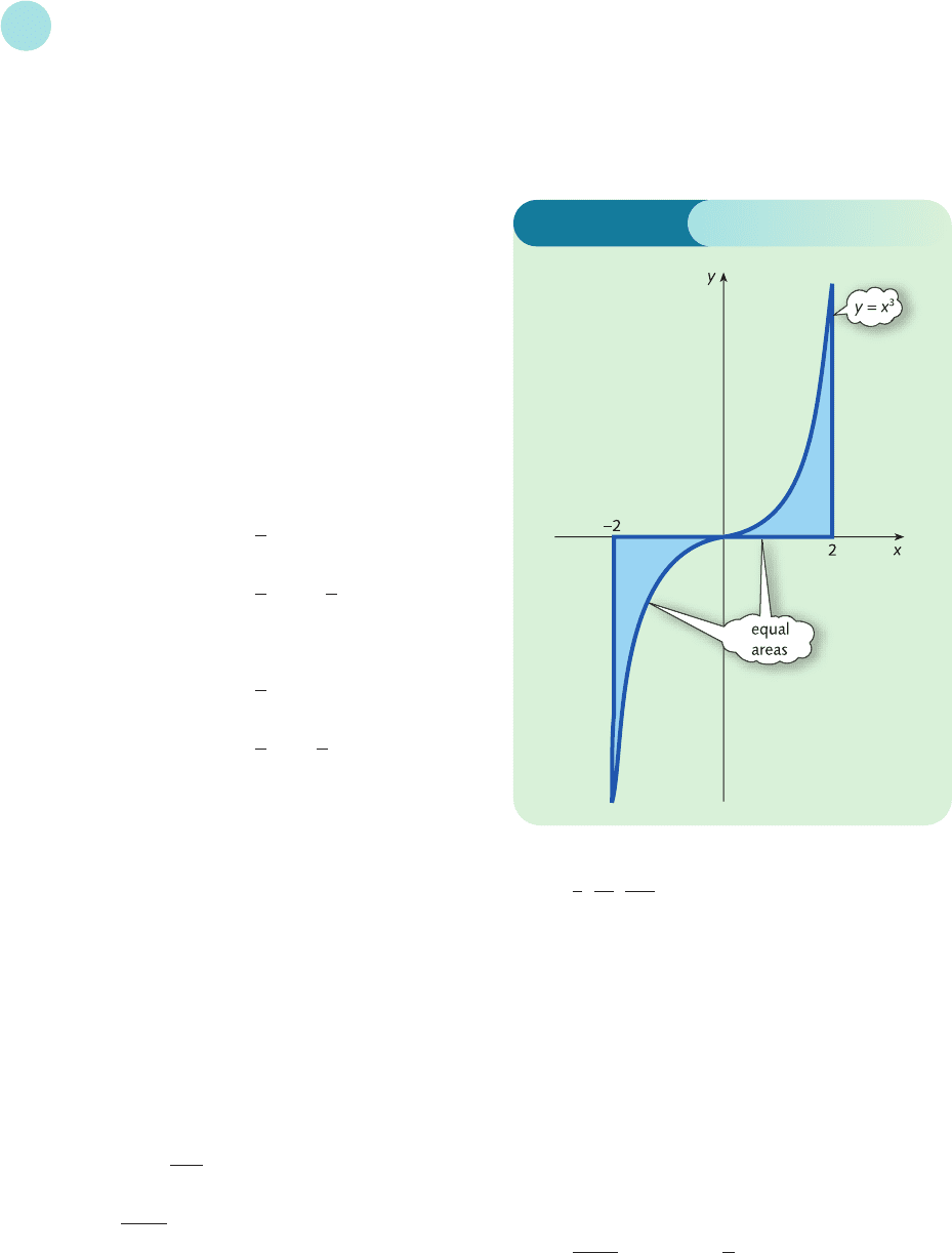
7 (a) 4; (b) 0. The graph is sketched in Figure S6.1.
Integration gives a positive value when the graph is
5000
0.06
J
L
1
0.06
G
I
J
L
3
4
3
4
G
I
J
L
3
4
G
I
J
L
3
4
3
4
G
I
J
L
3
4
G
I
8 (a) , , ; 1.
(b) 2√2 − 2, 2√20 − 2, 2√200 − 2; integral does not
exist because these numbers are increasing
without bound.
9 (a) 1.367 544 468, 1.8, 1.936 754 441; 2.
(b) 9, 99, 999; integral does not exist because these
numbers are increasing without bound.
10 (a) 100; (b) 20.
11 (a) 81; (b) 180.
12 (a) 74.67; (b) 58.67.
13 (a) $427.32; (b) During the 47th year.
14 (a) ; (b) (e
αT
− 1)
15 (a) $2785.84; (b) $7869.39;
(c) $19 865.24; (d) $20 000.
16 6.9 years.
A
α
AT
α+1
α+1
199
200
19
20
1
2
Solutions to Problems
646
Figure S6.1
above the x axis and a negative value when it is below
the x axis. In this case there are equal amounts of
positive and negative area which cancel out. Actual
area is twice that between 0 and 2, so is 8.
MFE_Z02.qxd 16/12/2005 10:51 Page 646

Chapter 7
Section 7.1
1 (a) 2 × 2, 1 × 5, 3 × 5, 1 × 1.
(b) 1, 4, 6, 2, 6, ?, 6; the value of c
43
does not exist,
because C has only three rows.
2A
T
=
B
T
=
C
T
==C
Matrices with the property that C
T
= C are called
symmetric. Elements in the top right-hand corner
are a mirror image of those in the bottom left-hand
corner.
3 (a) ; (c) ; (d) ; (e) .
Part (b) is impossible because A and C have different
orders.
4 (1) (a) ; (b) ;
(c) ; (d) .
From (a) and (b)
2A + 2B =+=
which is the same as (d), so
2(A + B) = 2A + 2B
(2) (a) ; (b) .
J
K
K
L
−6 12
−18 −30
0 −24
G
H
H
I
J
K
K
L
3 −6
915
012
G
H
H
I
J
K
K
L
2 −6
10 24
220
G
H
H
I
J
K
K
L
0 −2
414
212
G
H
H
I
J
K
K
L
2 −4
610
08
G
H
H
I
J
K
K
L
2
−6
10 24
220
G
H
H
I
J
K
K
L
1 −3
512
110
G
H
H
I
J
K
K
L
2 −2
414
212
G
H
H
I
J
K
K
L
2 −4
610
08
G
H
H
I
J
K
L
00
00
G
H
I
J
K
L
2
2
G
H
I
J
K
L
3
2
G
H
I
J
K
L
17
3 −8
G
H
I
J
K
K
L
123
245
356
G
H
H
I
J
K
K
K
L
1
5
7
9
G
H
H
H
I
J
K
K
K
K
K
L
1322
47 1−5
0631
1158
24−10
G
H
H
H
H
H
I
From (a),
−2(3A) =−2 =
which is the same as (b), so
−2(3A) =−6A
5 (a) [8] because
1(0) + (−
1)(−1)
+ 0(1) + 3(1) + 2(2) = 8
(b) [0] because 1(−2) + 2(1) + 9(0) = 0.
(c) This is impossible, because a and d have different
numbers of elements.
6
AB ==
AB ==
AB ==
AB ==
AB ==
AB ==
AB ==
J
K
K
L
710
34
610
G
H
H
I
J
K
L
12
34
G
H
I
J
K
K
L
12
01
31
G
H
H
I
J
K
K
L
710
34
6 c
32
G
H
H
I
J
K
L
12
34
G
H
I
J
K
K
L
12
01
31
G
H
H
I
J
K
K
L
710
34
c
31
c
32
G
H
H
I
J
K
L
12
34
G
H
I
J
K
K
L
12
01
31
G
H
H
I
J
K
K
L
710
3 c
22
c
31
c
32
G
H
H
I
J
K
L
12
34
G
H
I
J
K
K
L
12
01
31
G
H
H
I
J
K
K
L
710
c
21
c
22
c
31
c
32
G
H
H
I
J
K
L
12
34
G
H
I
J
K
K
L
12
01
31
G
H
H
I
J
K
K
L
7 c
12
c
21
c
22
c
31
c
32
G
H
H
I
J
K
L
12
34
G
H
I
J
K
K
L
12
01
31
G
H
H
I
J
K
K
L
c
11
c
12
c
21
c
22
c
31
c
32
G
H
H
I
J
K
L
12
34
G
H
I
J
K
K
L
12
01
31
G
H
H
I
J
K
K
L
−6 12
−18 −30
0 −24
G
H
H
I
J
K
K
L
3 −6
915
012
G
H
H
I
Solutions to Problems
647
MFE_Z02.qxd 16/12/2005 10:51 Page 647

7 (a) ; (d) ; (f) ;
(g) ; (h) .
Parts (b), (c) and (e) are impossible because, in each
case, the number of columns in the first matrix is not
equal to the number of rows in the second.
8Axis the 3 × 1 matrix
However, x + 4y + 7z =−3, 2x + 6y + 5z = 10 and
8x + 9y + 5z = 1, so this matrix is just
which is b. Hence Ax = b.
9 (a) J = ; F = .
(b)
(c)
10 (a)
(b)
(c)
(d) Same answer as (c).
11 (a)
Total cost charged to each customer.
(b)
J
K
L
1372322
3145
G
H
I
J
K
L
5900
1100
G
H
I
J
K
K
L
4202030
6 2 10 10
24 22 26 14
G
H
H
I
J
K
K
L
2141812
42010
12 8 10 6
G
H
H
I
J
K
K
L
46218
2 0 10 0
12 14 16 8
G
H
H
I
J
K
L
41010
17 10 8
G
H
I
J
K
L
66 44 16
67 68 40
G
H
I
J
K
L
31 17 3
25 29 16
G
H
I
J
K
L
35 27 13
42 39 24
G
H
I
J
K
K
L
−3
10
1
G
H
H
I
J
K
K
L
x + 4y + 7z
2z + 6y + 5z
8x + 9y + 5z
G
H
H
I
J
K
L
56
11 15
G
H
I
J
K
K
L
57 9
33 3
6912
G
H
H
I
J
K
L
9613
27 15 28
G
H
I
J
K
K
L
43
2 −1
55
G
H
H
I
J
K
K
L
5
7
5
G
H
H
I
Amount of raw materials used to manufacture
each customer’s goods.
(c)
Total raw material costs to manufacture one item
of each good.
(d)
Total raw material costs to manufacture requisite
number of goods for each customer.
(e)
[7000]
Total revenue received from customers.
(f) [1210]
Total cost of raw materials.
(g) [5790]
Profit before deduction of labour, capital and
overheads.
12 (1) (a)
(b)
(c)
(d)
(A + B)
T
= A
T
+ B
T
: that is, ‘transpose of the sum is the
sum of the transposes’.
(2) (a)
(b)
(c)
(d)
(CD)
T
= D
T
C
T
: that is ‘transpose of a product is
the product of the transposes multiplied in reverse
order’.
J
K
K
L
−21
15
49
G
H
H
I
J
K
L
−214
159
G
H
I
J
K
K
L
2 −1
10
01
G
H
H
I
J
K
L
15
49
G
H
I
J
K
L
25 2
1510
G
H
I
J
K
K
L
21
55
210
G
H
H
I
J
K
L
12−3
−11 4
G
H
I
J
K
L
135
246
G
H
I
J
K
L
1005
205
G
H
I
J
K
K
L
35
75
30
G
H
H
I
Solutions to Problems
648
MFE_Z02.qxd 16/12/2005 10:51 Page 648

13 (a) B + C =
so A(B + C) =
AB = and
AC = , so
AB + AC =
(b) AB = , so
(AB)C =
BC = , so
A(BC) =
14 AB = [−3]; BA =
15 (a) AI ===A
Similarly, IA = A.
(b) A
−1
A
=
=
==
Similarly, AA
−1
= I.
(c) Ix ===x
16 (a) 7x + 5y
x + 3y
(b) A = , x = , b = .
J
K
K
L
6
3
1
G
H
H
I
J
K
K
L
x
y
z
G
H
H
I
J
K
K
L
23−2
1 −12
425
G
H
H
I
J
K
L
x
y
G
H
I
J
K
L
x
y
G
H
I
J
K
L
10
01
G
H
I
J
K
L
10
01
G
H
I
J
K
L
ad − bc 0
0 ad − bc
G
H
I
1
ad − bc
J
K
L
da − bc db − bd
−ca + ac −cb + ad
G
H
I
1
ad − bc
J
K
L
ab
cd
G
H
I
J
K
L
d −b
−ca
G
H
I
1
ad − bc
J
K
L
ab
cd
G
H
I
J
K
L
10
01
G
H
I
J
K
L
ab
cd
G
H
I
J
K
K
K
L
12−40
714−28 21
36−12 9
−2 −48−6
G
H
H
H
I
J
K
L
32 43
426
G
H
I
J
K
L
411
−44
G
H
I
J
K
L
32 43
426
G
H
I
J
K
L
−725
610
G
H
I
J
K
L
−15 24
514
G
H
I
J
K
L
−8 −1
−14
G
H
I
J
K
L
−725
610
G
H
I
J
K
L
−15 24
514
G
H
I
J
K
L
06
52
G
H
I
Section 7.2
1 | A|=6(2) − 4(1) = 8 ≠ 0
so A is non-singular and its inverse is given by
=
| B |=6(2) − 4(3) = 0
so B is singular and its inverse does not exist.
2 We need to solve Ax = b, where
A = x = b =
Now
A
−1
=
so
==
3 In equilibrium, Q
S
= Q
D
= Q, say, so the supply
equation becomes
P = aQ + b
Subtracting aQ from both sides gives
P − aQ = b (1)
Similarly, the demand equation leads to
P + cQ = d (2)
In matrix notation equations (1) and (2) become
=
The coefficient matrix has an inverse,
so that
=
that is,
P = and Q =
The multiplier for Q due to changes in b is given
by the (2, 1) element of the inverse matrix so is
−1
c + a
−b + d
c + a
cb + ad
c + a
J
K
L
b
d
G
H
I
J
K
L
ca
−1 1
G
H
I
1
c + a
J
K
L
P
Q
G
H
I
J
K
L
ca
−1 1
G
H
I
1
c + a
J
K
L
b
d
G
H
I
J
K
L
P
Q
G
H
I
J
K
L
1 −a
1 c
G
H
I
J
K
L
4
7
G
H
I
J
K
L
43
57
G
H
I
J
K
L
7 −1
−2 9
G
H
I
1
61
J
K
L
P
1
P
2
G
H
I
J
K
L
7 −1
−2 9
G
H
I
1
61
J
K
L
43
57
G
H
I
J
K
L
P
1
P
2
G
H
I
J
K
L
91
27
G
H
I
J
K
L
1/4 −1/2
−1/8 3/4
G
H
I
J
K
L
2 −4
−1 −6
G
H
I
1
8
Solutions to Problems
649
MFE_Z02.qxd 16/12/2005 10:51 Page 649