Jacques I. Mathematics for Economics and Business

Подождите немного. Документ загружается.

14 Find expressions for

(a)

for the supply function Q = P

+ P + 1

(b) for the total revenue function TR = 50Q − 3Q

(d) for the consumption function C = 3Y + 7

(e) for the production function Q = 10 L

(f) for the proﬁt function π=−2Q

+ 15Q

− 24Q − 3

dπ

d(AC)

d(TR)

Differentiation

260

MFE_C04b.qxd 16/12/2005 11:11 Page 260

section 4.3

Marginal functions

At this stage you may be wondering what on earth differentiation has got to do with economics.

In fact, we cannot get very far with economic theory without making use of calculus. In this

section we concentrate on three main areas that illustrate its applicability:

 revenue and cost

 production

 consumption and savings.

We consider each of these in turn.

4.3.1 Revenue and cost

In Chapter 2 we investigated the basic properties of the revenue function, TR. It is deﬁned to

be PQ, where P denotes the price of a good and Q denotes the quantity demanded. In practice,

we usually know the demand equation, which provides a relationship between P and Q. This

enables a formula for TR to be written down solely in terms of Q. For example, if

P = 100 − 2Q

Objectives

At the end of this section you should be able to:

 Calculate marginal revenue and marginal cost.

 Derive the relationship between marginal and average revenue for both a

monopoly and perfect competition.

 Calculate marginal product of labour.

 State the law of diminishing marginal productivity using the notation of calculus.

 Calculate marginal propensity to consume and marginal propensity to save.

MFE_C04c.qxd 16/12/2005 11:12 Page 261

Differentiation

262

then

TR = PQ

= (100 − 2Q)Q

= 100Q − 2Q

The formula can be used to calculate the value of TR corresponding to any value of Q. Not

content with this, we are also interested in the effect on TR of a change in the value of Q from

some existing level. To do this we introduce the concept of marginal revenue. The marginal

revenue, MR, of a good is deﬁned by

MR =

marginal revenue is the derivative of total revenue with respect to demand

For example, the marginal revenue function corresponding to

TR = 100Q − 2Q

is given by

= 100 − 4Q

If the current demand is 15, say, then

MR = 100 − 4(15) = 40

You may be familiar with an alternative deﬁnition often quoted in elementary economics

textbooks. Marginal revenue is sometimes taken to be the change in TR brought about by a

1 unit increase in Q. It is easy to check that this gives an acceptable approximation to MR,

although it is not quite the same as the exact value obtained by differentiation. For example,

substituting Q = 15 into the total revenue function considered previously gives

TR = 100(15) − 2(15)

= 1050

An increase of 1 unit in the value of Q produces a total revenue

TR = 100(16) − 2(16)

= 1088

This is an increase of 38, which, according to the non-calculus deﬁnition, is the value of MR

when Q is 15. This compares with the exact value of 40 obtained by differentiation.

It is instructive to give a graphical interpretation of these two approaches. In Figure 4.14 the

point A lies on the TR curve corresponding to a quantity Q

. The exact value of MR at this point

is equal to the derivative

and so is given by the slope of the tangent at A. The point B also lies on the curve but cor-

responds to a 1 unit increase in Q. The vertical distance from A to B therefore equals the change

in TR when Q increases by 1 unit. The slope of the chord joining A and B is

==∆(TR)

∆(TR)

∆Q

d(TR)

MFE_C04c.qxd 16/12/2005 11:12 Page 262

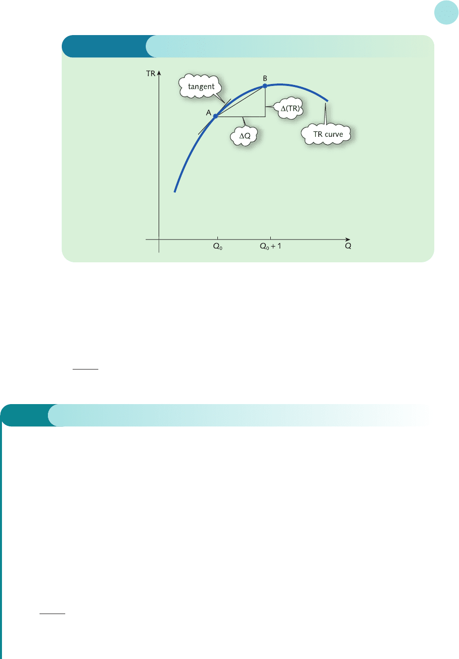
In other words, the slope of the chord is equal to the value of MR obtained from the non-

calculus deﬁnition. Inspection of the diagram reveals that the slope of the tangent is approxi-

mately the same as that of the chord joining A and B. In this case the slope of the tangent is

slightly the larger of the two, but there is not much in it. We therefore see that the 1 unit

increase approach produces a reasonable approximation to the exact value of MR given by

d(TR)

4.3 • Marginal functions

263

Figure 4.14

Example

If the demand function is

P = 120 − 3Q

ﬁnd an expression for TR in terms of Q.

Find the value of MR at Q = 10 using

(a) differentiation

(b) the 1 unit increase approach

Solution

TR = PQ = (120 − 3Q)Q = 120Q − 3Q

(a) The general expression for MR is given by

= 120 − 6Q

so at Q

10,

MR = 120 − 6 × 10 = 60

d(TR)



MFE_C04c.qxd 16/12/2005 11:12 Page 263

(b) From the non-calculus deﬁnition we need to ﬁnd the change in TR as Q increases from 10 to 11.

Putting Q = 10 gives TR = 120 × 10 − 3 × 10

= 900

Putting Q = 11 gives TR = 120 × 11 − 3 × 11

= 957

and so MR  57

Differentiation

264

Practice Problem

1 If the demand function is

P = 60 − Q

find an expression for TR in terms of Q.

(1) Differentiate TR with respect to Q to find a general expression for MR in terms of Q. Hence write

down the exact value of MR at Q = 50.

(2) Calculate the value of TR when

(a)

Q = 50 (b) Q = 51

and hence confirm that the 1 unit increase approach gives a reasonable approximation to the exact

value of MR obtained in part (1).

The approximation indicated by Figure 4.14 holds for any value of ∆Q. The slope of the

tangent at A is the marginal revenue, MR. The slope of the chord joining A and B is ∆(TR)/∆Q.

It follows that

MR 

This equation can be transposed to give

∆(TR)  MR ×∆Q

that is,

 ×

Moreover, Figure 4.14 shows that the smaller the value of ∆Q, the better the approximation

becomes. This, of course, is similar to the argument used at the end of Section 4.1 when we

discussed the formal deﬁnition of a derivative as a limit.

change in

demand

marginal

revenue

change in

total revenue

∆(TR)

∆Q

Example

If the total revenue function of a good is given by

100Q − Q

write down an expression for the marginal revenue function. If the current demand is 60, estimate the

change in the value of TR due to a 2 unit increase in Q.

MFE_C04c.qxd 16/12/2005 11:12 Page 264

Solution

TR = 100Q − Q

then

MR =

= 100 − 2Q

When Q = 60

MR = 100 − 2(60) =−20

If Q increases by 2 units, ∆Q = 2 and the formula

∆(TR)  MR ×∆Q

shows that the change in total revenue is approximately

(−20) × 2 =−40

A 2 unit increase in Q therefore leads to a decrease in TR of about 40.

d(TR)

4.3 • Marginal functions

265

Practice Problem

2 If the total revenue function of a good is given by

1000Q − 4Q

write down an expression for the marginal revenue function. If the current demand is 30, find the

approximate change in the value of TR due to a

(a) 3 unit increase in Q

(b) 2 unit decrease in Q

The simple model of demand, originally introduced in Section 1.3, assumed that price, P,

and quantity, Q, are linearly related according to an equation

P = aQ + b

where the slope, a, is negative and the intercept, b, is positive. A downward-sloping demand

curve such as this corresponds to the case of a monopolist. A single ﬁrm, or possibly a group of

ﬁrms forming a cartel, is assumed to be the only supplier of a particular product and so has

control over the market price. As the ﬁrm raises the price, so demand falls. The associated total

revenue function is given by

TR = PQ

= (aQ + b)Q

= aQ

+ bQ

An expression for marginal revenue is obtained by differentiating TR with respect to Q to get

MR = 2aQ + b

MFE_C04c.qxd 16/12/2005 11:12 Page 265

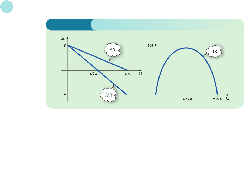
It is interesting to notice that, on the assumption of a linear demand equation, the marginal

revenue is also linear with the same intercept, b, but with slope 2a. The marginal revenue curve

slopes downhill exactly twice as fast as the demand curve. This is illustrated in Figure 4.15(a).

The average revenue, AR, is deﬁned by

AR =

and, since TR = PQ, we have

AR ==P

For this reason the demand curve is labelled average revenue in Figure 4.15(a). The above

derivation of the result AR = P is independent of the particular demand function. Con-

sequently, the terms ‘average revenue curve’ and ‘demand curve’ are synonymous.

Figure 4.15(a) shows that the marginal revenue takes both positive and negative values. This

is to be expected. The total revenue function is a quadratic and its graph has the familiar

parabolic shape indicated in Figure 4.15(b). To the left of −b/2a the graph is uphill, corres-

ponding to a positive value of marginal revenue, whereas to the right of this point it is down-

hill, giving a negative value of marginal revenue. More signiﬁcantly, at the maximum point of

the TR curve, the tangent is horizontal with zero slope and so MR is zero.

At the other extreme from a monopolist is the case of perfect competition. For this model we

assume that there are a large number of ﬁrms all selling an identical product and that there are

no barriers to entry into the industry. Since any individual ﬁrm produces a tiny proportion of

the total output, it has no control over price. The ﬁrm can sell only at the prevailing market

price and, because the ﬁrm is relatively small, it can sell any number of goods at this price.

If the ﬁxed price is denoted by b then the demand function is

P = b

and the associated total revenue function is

TR = PQ = bQ

An expression for marginal revenue is obtained by differentiating TR with respect to Q and,

since b is just a constant, we see that

MR = b

In the case of perfect competition, the average and marginal revenue curves are the same. They

are horizontal straight lines, b units above the Q axis as shown in Figure 4.16.

Differentiation

266

Figure 4.15

MFE_C04c.qxd 16/12/2005 11:12 Page 266

4.3 • Marginal functions

267

Figure 4.16

Example

If the average cost function of a good is

AC = 2Q + 6 +

ﬁnd an expression for MC. If the current output is 15, estimate the effect on TC of a 3 unit decrease in Q.

Solution

We ﬁrst need to ﬁnd an expression for TC using the given formula for AC. Now we know that the average

cost is just the total cost divided by Q: that is,

AC =

So far we have concentrated on the total revenue function. Exactly the same principle can be

used for other economic functions. For instance, we deﬁne the marginal cost, MC, by

MC =

marginal cost is the derivative of total cost with respect to output

Again, using a simple geometrical argument, it is easy to see that if Q changes by a small

amount ∆Q then the corresponding change in TC is given by

∆(TC)  MC ×∆Q

 ×

In particular, putting ∆Q = 1 gives

∆(TC)  MC

so that MC gives the approximate change in TC when Q increases by 1 unit.

change in

output

marginal

cost

change in

total cost

d(TC)

MFE_C04c.qxd 16/12/2005 11:12 Page 267

Hence

TC = (AC)Q

= 2Q + 6 + Q

and, after multiplying out the brackets, we get

TC = 2Q

+ 6Q + 13

In this formula the last term, 13, is independent of Q so must denote the ﬁxed costs. The

remaining part, 2Q

+ 6Q, depends on Q so represents the total variable costs. Differentiating

gives

MC =

= 4Q + 6

Notice that because the ﬁxed costs are constant they differentiate to zero and so have no effect

on the marginal cost. When Q = 15,

MC = 4(15) + 6 = 66

Also, if Q decreases by 3 units then ∆Q =−3. Hence the change in TC is given by

∆(TC)  MC ×∆Q

= 66 × (−3)

=−198

so TC decreases by 198 units approximately.

d(TC)

Differentiation

268

Practice Problem

3 Find the marginal cost given the average cost function

AC =+2

Deduce that a 1 unit increase in Q will always result in a 2 unit increase in TC, irrespective of the

current level of output.

100

4.3.2 Production

Production functions were introduced in Section 2.3. In the simplest case output, Q, is

assumed to be a function of labour, L, and capital, K. Moreover, in the short run the input K

can be assumed to be ﬁxed, so Q is then only a function of one input L. (This is not a valid

assumption in the long run and in general Q must be regarded as a function of at least two

inputs. Methods for handling this situation are considered in the next chapter.) The variable L

is usually measured in terms of the number of workers or possibly in terms of the number

of worker hours. Motivated by our previous work, we deﬁne the marginal product of labour,

, by

MFE_C04c.qxd 16/12/2005 11:12 Page 268

4.3 • Marginal functions

269

Example

If the production function is

Q = 300 L − 4L

where Q denotes output and L denotes the size of the workforce, calculate the value of MP

when

(a) L = 1

(b) L = 9

(d) L = 2500

and discuss the implications of these results.

Solution

Q = 300 L − 4L = 300L

1/ 2

− 4L

then

= 300(

/2 L

−1/ 2

) − 4

= 150L

−1/ 2

− 4

=−4

(a) When L = 1

=−4 = 146

(b) When L = 9

=−4 = 46

=−4 = 11

(d) When L = 2500

=−4 =−1

150

2500

150

100

150



marginal product of labour is the derivative of output with respect to labour

As before, this gives the approximate change in Q that results from using 1 more unit of L.

MFE_C04c.qxd 16/12/2005 11:12 Page 269