Jacques I. Mathematics for Economics and Business
Подождите немного. Документ загружается.


it is virtually impossible to obtain the exact solution. The best way of proceeding would be to use a non-
linear equation-solver routine on a computer, particularly if it is important that an accurate value of r
is obtained. However, if all that is needed is a rough approximation then this can be done by systematic
trial and error. We merely substitute likely solutions into the right-hand side of the equation until we
find the one that works. For example, putting r = 5 gives
++=5358
Other values of the expression
1000 1 +
−1
+ 2000 1 +
−2
+ 3000 1 +
−3
corresponding to r = 6, 7,..., 10 are listed in the following table:
r 678910
value 5242 5130 5022 4917 4816
Given that we are trying to find r so that this value is 5000, this table indicates that r is some-
where between 8% (which produces a value greater than 5000) and 9% (which produces a value less
than 5000).
If a more accurate estimate of IRR is required then we simply try further values between 8% and 9%.
For example, it is easy to check that putting r = 8
1
/
2 gives 4969, indicating that the exact value of r is
between 8% and 8
1
/2%. We conclude that the IRR is 8% to the nearest percentage.
D
F
r
100
A
C
D
F
r
100
A
C
D
F
r
100
A
C
3000
(1.05)
3
2000
(1.05)
2
1000
1.05
Mathematics of Finance
230
Practice Problem
6 A project requires an initial investment of $12 000. It has a guaranteed return of $8000 at the end of
year 1 and a return of $2000 each year at the end of years 2, 3 and 4.
Estimate the IRR to the nearest percentage. Would you recommend that someone invests in this
project if the prevailing market rate is 8% compounded annually?
Problem 6 should have convinced you how tedious it is to calculate the internal rate of
return ‘by hand’ when there are more than two payments in a revenue flow. A computer
spreadsheet provides the ideal tool for dealing with this. Chart Wizard can be used to sketch a
graph from which a rough estimate of IRR can be found. A more accurate value can be found
using a ‘finer’ tabulation in the vicinity of this estimate.
Example
A proposed investment project costs $11 600 today. The expected revenue flow (in thousands of dollars) for
the next 4 years is
Year 1234
Revenue flow 2 3.7 3.8 4.5
Use a graphical method to determine the IRR to the nearest whole number. By tabulating further values,
estimate the IRR correct to 1 decimal place.
EXCEL
MFE_C03d.qxd 16/12/2005 11:03 Page 230
Solution
Before we tackle this particular example, it will be useful to review the definition of the internal rate of
return. So far, we have taken it to be the rate of interest at which the total present values of the revenue
stream equal the initial outlay. Of course, this is the same as saying that the difference between present
values and the initial outlay is zero. In other words, the internal rate of return is the interest rate which gives
a net present value (NPV) of zero. We shall exploit this fact by plotting a graph of net present values against
interest rate (r). The IRR is the value of r at which the graph crosses the horizontal axis.
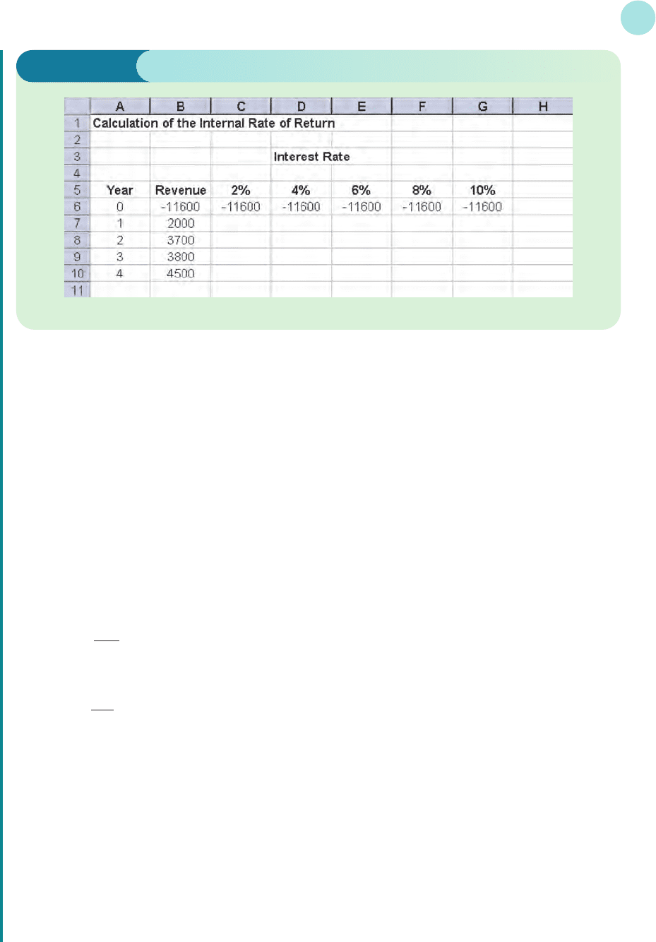
We begin by typing suitable headings together with values of the years and revenue flows for this project
into a spreadsheet, as shown in Figure 3.4.
Notice that the initial investment in the project has been input as a negative number, since this represents
an outflow of funds. The present value of this is also −11 600, since this occurs in year 0. The columns
represent interest rates of 2%, 4%,..., 10%. The values in the body of the table will be the present values
of the revenue flows, calculated at each of these rates of interest. For example, the entry in cell C7 will be the
present value of the $2000 received at the end of year 1 when the interest rate is 2%. From the formula
P = S 1 +
−t
this is
2000 1 +
−1
Notice that the numbers 2000 and 1 appear in cells B7 and A7, respectively, so the formula that we need for
cell C7 is
=B7*(1.02)^(-A7)
By clicking and dragging this formula down to C10, we complete the present values for the 2% interest rate.
For the next column, we simply change the scale factor 1.02 to 1.04, so we type
=B7*(1.04)^(-A7)
in cell D7 and repeat the process. We can obviously continue in this way along the rest of the table. Finally,
we calculate the net present values by summing the entries for the present values in each column. For
example, to find the NPV for the 2% interest rate we type
D
F
2
100
A
C
D
F
r
100
A
C
3.4 • Investment appraisal
231
Figure 3.4
MFE_C03d.qxd 16/12/2005 11:03 Page 231
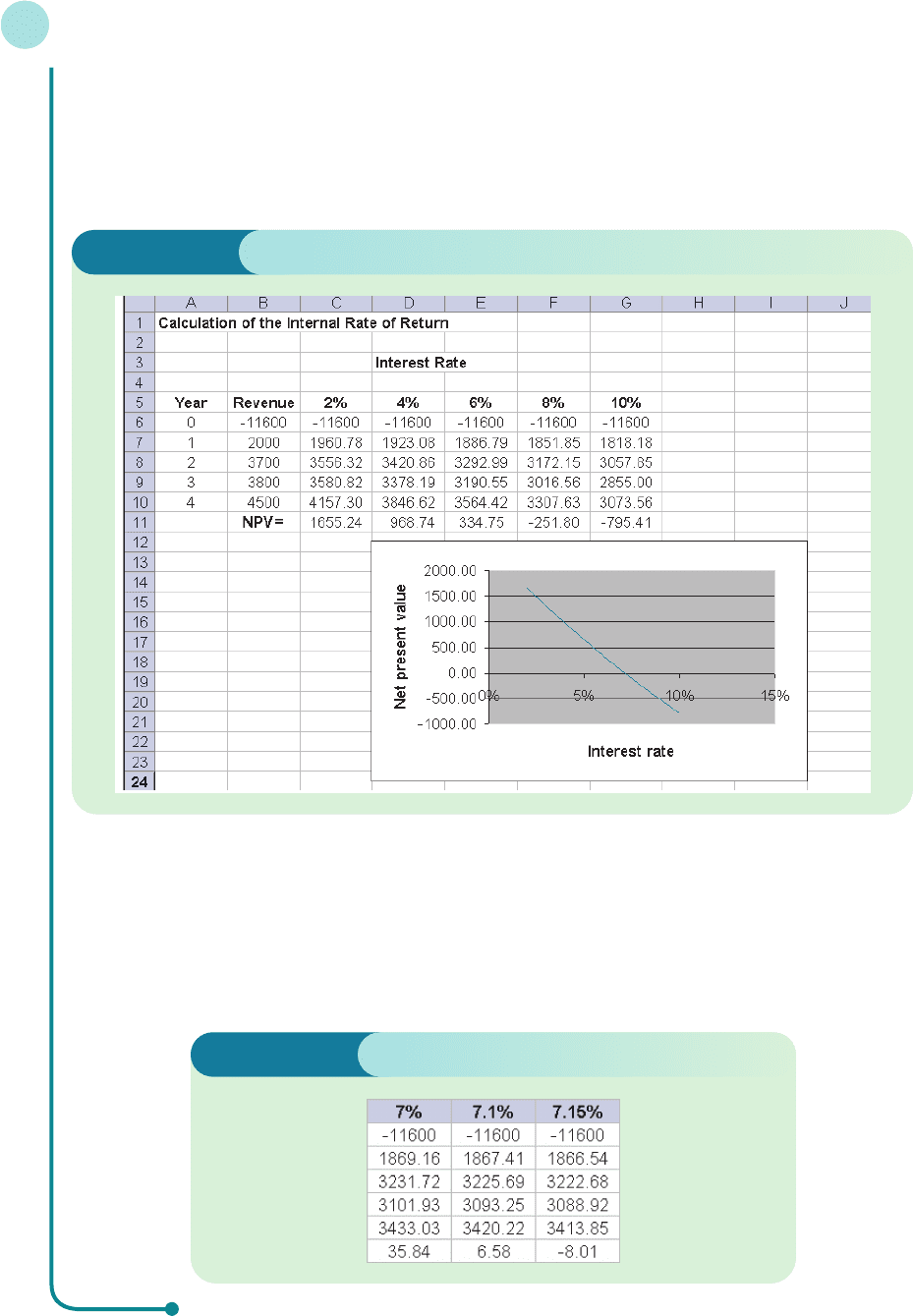
=SUM(C6:C10)
in cell C11. (A quicker way of doing this is just to highlight cells C6 to C11 and click on the ∑ icon on the
toolbar. This is the Greek letter sigma, which mathematicians use as an abbreviation for SUM. Excel will
then sum these five cells and put the answer in C11.) Figure 3.5 shows the completed spreadsheet. The
values have been rounded to 2 decimal places using the Decrease Decimal button on the toolbar.
Mathematics of Finance
232
Figure 3.5
Figure 3.6
A graph of NPV against r is shown in Figure 3.5. This is plotted by highlighting the cells in rows 5 and
11, and using Chart Wizard. (Click and drag from C5 to G5 then, holding down the Ctrl key, click and drag
from C11 to G11.) The graph shows that to the nearest whole number, the internal rate of return is 7%.
To obtain a more accurate estimate of IRR, we return to the spreadsheet and add more columns for inter-
est rates near 7%. By looking at the bottom row of the table in Figure 3.6 we see that, to 1 decimal place, the
IRR is 7.1%.
MFE_C03d.qxd 16/12/2005 11:03 Page 232

We conclude this section by using the theory of discounting to explain the relationship
between interest rates and the speculative demand for money. This was first introduced in
Section 1.6 in the analysis of LM schedules. Speculative demand consists of money held in
reserve to take advantage of changes in the value of alternative financial assets, such as govern-
ment bonds. As their name suggests, these issues can be bought from the government at a cer-
tain price. In return, the government pays out interest on an annual basis for a prescribed
number of years. At the end of this period the bond is redeemed and the purchaser is repaid
the original sum. Now these bonds can be bought and sold at any point in their lifetime. The
person who chooses to buy one of these bonds part-way through this period is entitled to all of
the future interest payments, together with the final redemption payment. The value of exist-
ing securities clearly depends on the number of years remaining before redemption, together
with the prevailing rate of interest.
3.4 • Investment appraisal
233
Example
A 10-year bond is originally offered by the government at $5000 with an annual return of 9%. Assuming
that the bond has 4 years left before redemption, calculate its present value assuming that the prevailing
interest rate is
(a) 5% (b) 7% (c) 9% (d) 11% (e) 13%
Solution
The government pays annual interest of 9% on the $5000 bond, so agrees to pay the holder $450 every year
for 10 years. At the end of the 10 years, the bond is redeemed by the government and $5000 is paid back to
the purchaser. If there are just 4 years left between now and the date of redemption, the future cash flow
that is paid on the bond is summarized in the second column of Table 3.22. This is similar to that of an
annuity except that in the final year an extra payment of $5000 is received when the government pays back
the original investment. The present value of this income stream is calculated in Table 3.22 using the given
discount rates of 5%, 7%, 9%, 11% and 13% compounded annually. The total present value in each case is
given in the last row of this table and varies from $5710 when the interest rate is 5% to $4405 when it is 13%.
Notice from the table in the previous example that the value of a bond falls as interest rates rise. This is
entirely to be expected, since the formula we use to calculate individual present values is
P =
and larger values of r produce smaller values of P.
S
(1 + r/100)
t
Table 3.22
Present values
End of year Cash flow 5% 7% 9% 11% 13%
1 450 429 421 413 405 398
2 450 408 393 379 365 352
3 450 389 367 347 329 312
4 5450 4484 4158 3861 3590 3343
Total present value 5710 5339 5000 4689 4405
MFE_C03d.qxd 16/12/2005 11:03 Page 233

The effect of this relationship on financial markets can now be analysed. Let us suppose that the interest
rate is high at, say, 13%. As you can see from Table 3.22, the price of the bond is relatively low. Moreover,
one might reasonably expect that, in the future, interest rates are likely to fall, thereby increasing the
present value of the bond. In this situation an investor would be encouraged to buy this bond in the
expectation of not only receiving the cash flow from holding the bond but also receiving a capital gain on
its present value. Speculative balances therefore decrease as a result of high interest rates because money
is converted into securities. Exactly the opposite happens when interest rates are low. The corresponding
present value is relatively high, and, with an expectation of a rise in interest rates and a possible capital loss,
investors are reluctant to invest in securities, so speculative balances are high.
Mathematics of Finance
234
Practice Problem
7 A 10-year bond is originally offered by the government at $1000 with an annual return of 7%.
Assuming that the bond currently has 3 years left before redemption and that the prevailing interest
rate is 8% compounded annually, calculate its present value.
Annuity A lump sum investment designed to produce a sequence of equal regular pay-
ments over time.
Discount rate The interest rate that is used when going backwards in time to calculate the
present value from a future value.
Discounting The process of working backwards in time to find the present values from a
future value.
Internal rate of return The interest rate for which the net present value is zero.
Net present value The present value of a revenue flow minus the original cost.
Present value The amount that is invested initially to produce a specified future value after
a given period of time.
Key Terms
Practice Problems
8 Determine the present value of $7000 in 2 years’ time if the discount rate is 8% compounded
(a) quarterly (b) continuously
9 A small business promises a profit of $8000 on an initial investment of $20 000 after 5 years.
(a) Calculate the internal rate of return.
(b) Would you advise someone to invest in this business if the market rate is 6% compounded
annually?
10 You are given the opportunity of investing in one of three projects. Projects A, B and C require
initial outlays of $20 000, $30 000 and $100 000 and are guaranteed to return $25 000, $37 000 and
$117 000, respectively, in 3 years’ time. Which of these projects would you invest in if the market
rate is 5% compounded annually?
MFE_C03d.qxd 16/12/2005 11:03 Page 234

11 Determine the present value of an annuity that pays out $100 at the end of each year
(a) for 5 years (b) in perpetuity
if the interest rate is 10% compounded annually.
12 A firm decides to invest in a new piece of machinery which is expected to produce an additional rev-
enue of $8000 at the end of every year for 10 years. At the end of this period the firm plans to sell
the machinery for scrap, for which it expects to receive $5000. What is the maximum amount that
the firm should pay for the machine if it is not to suffer a net loss as a result of this investment? You
may assume that the discount rate is 6% compounded annually.
13 During the next 3 years a business decides to invest $10 000 at the beginning of each year. The cor-
responding revenue that it can expect to receive at the end of each year is given in Table 3.23.
Calculate the net present value if the discount rate is 4% compounded annually.
3.4 • Investment appraisal
235
14 A project requires an initial investment of $50 000. It produces a return of $40 000 at the end of year
1 and $30 000 at the end of year 2. Find the exact value of the internal rate of return.
15 A government bond that originally cost $500 with a yield of 6% has 5 years left before redemption.
Determine its present value if the prevailing rate of interest is 15%.
16 An annuity pays out $20 000 per year in perpetuity. If the interest rate is 5% compounded annually,
find
(a) the present value of the whole annuity
(b) the present value of the annuity for payments received, starting from the end of the thirtieth year
(c) the present value of the annuity of the first 30 years
17 An engineering company needs to decide whether or not to build a new factory. The costs of build-
ing the factory are $150 million initially, together with a further $100 million at the end of the
next 2 years. Annual operating costs are $5 million commencing at the end of the third year. Annual
revenue is predicted to be $50 million commencing at the end of the third year. If the interest rate
is 6% compounded annually, find
(a) the present value of the building costs
(b) the present value of the operating costs at the end of n years (n > 2)
(c) the present value of the revenue after n years (n > 2)
(d) the minimum value of n for which the net present value is positive
18 An annuity pays out $a per year in perpetuity. If the interest rate is r% compounded annually, show
that the present value of the whole annuity is 100a/r.
19 (Excel) A proposed investment project costs $970 000 today, and is expected to generate revenues
(in thousands of dollars) at the end of each of the following four years of 280, 450, 300, 220
Table 3.23
End of year Revenue ($)
1 5 000
2 20 000
3 50 000
MFE_C03d.qxd 16/12/2005 11:03 Page 235

respectively. Sketch a graph of net present values against interest rates, r, over the range 0 ≤ r ≤ 14.
Use this graph to estimate the internal rate of return, to the nearest whole number. Use a spreadsheet
to perform more calculations in order to calculate the value of the IRR, correct to 1 decimal place.
20 (Excel) A civil engineering company needs to buy a new excavator. Model A is expected to make
a loss of $60 000 at the end of the first year, but is expected to produce revenues of $24 000 and
$72 000 for the second and third years of operation. The corresponding figures for model B are
$96 000, $12 000 and $120 000, respectively. Use a spreadsheet to tabulate the revenue flows (using
negative numbers for the losses in the first year), together with the corresponding present values
based on a discount rate of 8% compounded annually. Find the net present value for each model.
Which excavator, if any, would you recommend buying?
What difference does it make if the discount rate is 8% compounded continuously?
Mathematics of Finance
236
MFE_C03d.qxd 16/12/2005 11:03 Page 236

chapter 4
Differentiation
This chapter provides a simple introduction to the general topic of calculus. In fact,
‘calculus’ is a Latin word and a literal translation of it is ‘stone’. Unfortunately, all
too many students interpret this as meaning a heavy millstone that they have
to carry around with them! However, as we shall see, the techniques of calculus
actually provide us with a quick way of performing calculations. (The process of
counting was originally performed using stones a long time ago.)
There are eight sections, which should be read in the order that they appear. It
should be possible to omit Sections 4.5 and 4.7 at a first reading and Section 4.6 can
be read any time after Section 4.3.
Section 4.1 provides a leisurely introduction to the basic idea of differentiation. The
material is explained using pictures, which will help you to understand the con-
nection between the underlying mathematics and the economic applications in later
sections.
There are six rules of differentiation, which are evenly split between Sections 4.2 and
4.4. Section 4.2 considers the easy rules that all students will need to know.
However, if you are on a business studies or accountancy course, or are on a
low-level economics route, then the more advanced rules in Section 4.4 may not be
of relevance and could be ignored. As far as possible, examples given in later sections
and chapters are based on the easy rules only so that such students are not dis-
advantaged. However, the more advanced rules are essential to any proper study of
mathematical economics and their use in deriving general results is unavoidable.
Sections 4.3 and 4.5 describe standard economic applications. Marginal functions
associated with revenue, cost, production, consumption and savings functions are all
MFE_C04a.qxd 16/12/2005 11:09 Page 237

discussed in Section 4.3. The important topic of elasticity is described in Section 4.5.
The distinction is made between price elasticity along an arc and price elasticity at a
point. Familiar results involving general linear demand functions and the relationship
between price elasticity of demand and revenue are derived.
Sections 4.6 and 4.7 are devoted to the topic of optimization, which is used to find
the maximum and minimum values of economic functions. In the first half of Section
4.6 we concentrate on the mathematical technique. The second half contains four
examination-type problems, all taken from economics, which are solved in detail. In
Section 4.7, mathematics is used to derive general results relating to the optimiza-
tion of profit and production functions.
The final section revises two important mathematical functions, namely the expon-
ential and natural logarithm functions. We describe how to differentiate these
functions and illustrate their use in economics.
Differentiation is probably the most important topic in the whole book, and one that
we shall continue in Chapters 5 and 6, since it provides the necessary background
theory for much of mathematical economics. You are therefore advised to make
every effort to attempt the problems given in each section. The prerequisites include
an understanding of the concept of a function together with the ability to manipu-
late algebraic expressions. These are covered in Chapters 1 and 2, and if you have
worked successfully through this material, you should find that you are in good
shape to begin calculus.
MFE_C04a.qxd 16/12/2005 11:09 Page 238

section 4.1
The derivative of a function
This introductory section is designed to get you started with differential calculus in a fairly pain-
less way. There are really only three things that we are going to do. We discuss the basic idea of
something called a derived function, give you two equivalent pieces of notation to describe it
and finally show you how to write down a formula for the derived function in simple cases.
In Chapter 1 the slope of a straight line was defined to be the change in the value of y brought
about by a 1 unit increase in x. In fact, it is not necessary to restrict the change in x to a 1 unit
increase. More generally, the slope, or gradient, of a line is taken to be the change in y divided
by the corresponding change in x as you move between any two points on the line. It is cus-
tomary to denote the change in y by ∆y, where ∆ is the Greek letter ‘delta’.
Likewise, the change in x is written ∆x. In this notation we have
slope =
∆y
∆x
Objectives
At the end of this section you should be able to:
Find the slope of a straight line given any two points on the line.
Detect whether a line is uphill, downhill or horizontal using the sign of the slope.
Recognize the notation f ′(x) and dy/dx for the derivative of a function.
Estimate the derivative of a function by measuring the slope of a tangent.
Differentiate power functions.
Example
Find the slope of the straight line passing through
(a) A (1, 2) and B (3, 4) (b) A (1, 2) and C (4, 1) (c) A (1, 2) and D (5, 2)
MFE_C04a.qxd 16/12/2005 11:09 Page 239