Jacques I. Mathematics for Economics and Business

Подождите немного. Документ загружается.

Non-linear Equations

130

Example

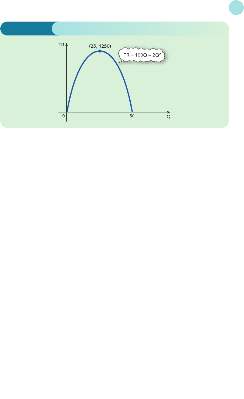
Given the demand function

P = 100 − 2Q

express TR as a function of Q and hence sketch its graph.

(a) For what values of Q is TR zero?

(b) What is the maximum value of TR?

Solution

Total revenue is deﬁned by

TR = PQ

and, since P = 100 − 2Q, we have

TR = (100 − 2Q)Q = 100Q − 2Q

This function is quadratic and so its graph can be sketched using the strategy described in Section 2.1.

Step 1

The coefﬁcient of Q

is negative, so the graph has an inverted U shape.

Step 2

The constant term is zero, so the graph crosses the TR axis at the origin.

Step 3

To ﬁnd where the curve crosses the horizontal axis, we could use ‘the formula’. However, this is not neces-

sary, since it follows immediately from the factorization

TR = (100 − 2Q)Q

that TR = 0 when either 100 − 2Q = 0 or Q = 0. In other words, the quadratic equation has two solutions,

Q = 0 and Q = 50.

The total revenue curve is shown in Figure 2.6.

 From Figure 2.6 the total revenue is zero when Q = 0 and Q = 50.

 By symmetry, the parabola reaches its maximum halfway between 0 and 50, that is at Q = 25. The

corresponding total revenue is given by

TR = 100(25) − 2(25)

= 1250

Practice Problem

1 Given the demand function

P = 1000 − Q

express TR as a function of Q and hence sketch a graph of TR against Q. What value of Q maximizes

total revenue and what is the corresponding price?

MFE_C02b.qxd 16/12/2005 10:59 Page 130

In general, given the linear demand function

P = aQ + b (a < 0, b > 0)

the total revenue function is

TR = PQ

= (aQ + b)Q

= aQ

+ bQ

This function is quadratic in Q and, since a < 0, the TR curve has an inverted U shape.

Moreover, since the constant term is zero, the curve always intersects the vertical axis at the ori-

gin. This fact should come as no surprise to you; if no goods are sold, the revenue must be zero.

We now turn our attention to the total cost function, TC, which relates the production costs

to the level of output, Q. As the quantity produced rises, the corresponding cost also rises, so

the TC function is increasing. However, in the short run, some of these costs are ﬁxed. Fixed

costs, FC, include the cost of land, equipment, rent and possibly skilled labour. Obviously, in

the long run all costs are variable, but these particular costs take time to vary, so can be thought

of as ﬁxed in the short run. Variable costs, on the other hand, vary with output and include the

cost of raw materials, components, energy and unskilled labour. If VC denotes the variable cost

per unit of output then the total variable cost, TVC, in producing Q goods is given by

TVC = (VC)Q

The total cost is the sum of the contributions from the ﬁxed and variable costs, so is given by

TC = FC + (VC)Q

Now although this is an important economic function, it does not always convey the informa-

tion necessary to compare individual ﬁrms. For example, suppose that an international car

company operates two plants, one in the USA and one in Europe, and suppose that the total

annual costs are known to be $200 million and $45 million respectively. Which of these two

plants is regarded as the more efﬁcient? Unfortunately, unless we also know the total number

of cars produced it is impossible to make any judgement. The signiﬁcant function here is not

the total cost, but rather the average cost per car. If the plants in the USA and Europe manu-

facture 80 000 and 15 000 cars, respectively, their corresponding average costs are

= 2500

200 000 000

80 000

2.2 • Revenue, cost and profit

131

Figure 2.6

MFE_C02b.qxd 16/12/2005 10:59 Page 131

and

= 3000

On the basis of these ﬁgures, the plant in the USA appears to be the more efﬁcient. In practice,

other factors would need to be taken into account before deciding to increase or decrease the

scale of operation in either country.

In general, the average cost function, AC, is obtained by dividing the total cost by output,

so that

AC =

=+VC

(VC)Q

FC + (VC)Q

45 000 000

15 000

Non-linear Equations

132

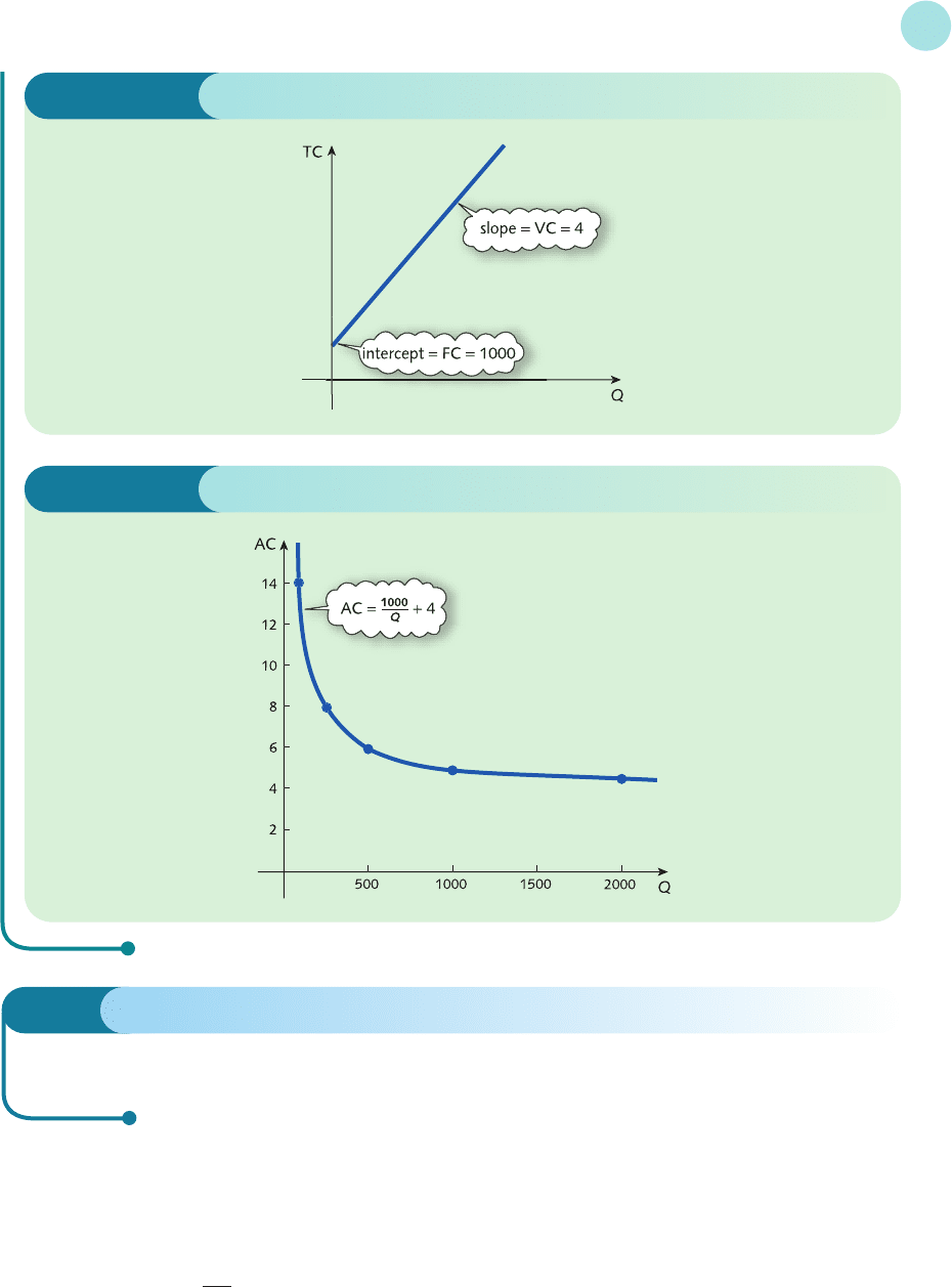
Example

Given that ﬁxed costs are 1000 and that variable costs are 4 per unit, express TC and AC as functions of Q.

Hence sketch their graphs.

Solution

We are given that FC = 1000 and VC = 4, so

TC = 1000 + 4Q

and

AC == = +4

The graph of the total cost function is easily sketched. It is a straight line with intercept 1000 and slope 4. It

is sketched in Figure 2.7. The average cost function is of a form that we have not met before, so we have no

prior knowledge about its basic shape. Under these circumstances it is useful to tabulate the function. The

tabulated values are then plotted on graph paper and a smooth curve obtained by joining the points

together. One particular table of function values is

Q 100 250 500 1000 2000

AC 14 8 6 5 4.5

These values are readily checked. For instance, when Q = 100

AC =+4 = 10 + 4 = 14

A graph of the average cost function, based on this table, is sketched in Figure 2.8. This curve is known as a

rectangular hyperbola and is sometimes referred to by economists as being L-shaped.

1000

100

1000

1000 + 4Q

MFE_C02b.qxd 16/12/2005 10:59 Page 132

In general, whenever the variable cost, VC, is a constant the total cost function,

TC = FC + (VC)Q

is linear. The intercept is FC and the slope is VC. For the average cost function

AC =+VC

note that if Q is small, then FC/Q is large, so the graph bends sharply upwards as Q approaches

zero. As Q increases, FC/Q decreases and eventually tails off to zero for large values of Q. The

2.2 • Revenue, cost and profit

133

Practice Problem

2 Given that fixed costs are 100 and that variable costs are 2 per unit, express TC and AC as functions

of Q. Hence sketch their graphs.

Figure 2.8

Figure 2.7

MFE_C02b.qxd 16/12/2005 10:59 Page 133

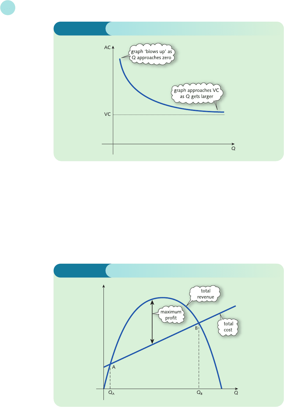
AC curve therefore ﬂattens off and approaches VC as Q gets larger and larger. This phe-

nomenon is hardly surprising, since the ﬁxed costs are shared between more and more goods,

so have little effect on AC for large Q. The graph of AC therefore has the basic L shape shown

in Figure 2.9. This discussion assumes that VC is a constant. In practice, this may not be the

case and VC might depend on Q. The TC graph is then no longer linear and the AC graph

becomes U-shaped rather than L-shaped. An example of this can be found in Practice Problem 7

at the end of this section.

Figure 2.10 shows typical TR and TC graphs sketched on the same diagram. These are drawn

on the assumption that the demand function is linear (which leads to a quadratic total revenue

Non-linear Equations

134

Figure 2.9

Figure 2.10

MFE_C02b.qxd 16/12/2005 10:59 Page 134

function) and that the variable costs are constant (which leads to a linear total cost function).

The horizontal axis represents quantity, Q. Strictly speaking the label Q means different things

for the two functions. For the revenue function, Q denotes the quantity of goods actually sold,

whereas for the cost function it denotes the quantity produced. In sketching both graphs on the

same diagram we are implicitly assuming that these two values are the same and that the ﬁrm

sells all of the goods that it produces.

The two curves intersect at precisely two points, A and B, corresponding to output levels Q

and Q

. At these points the cost and revenue are equal and the ﬁrm breaks even. If Q < Q

Q > Q

then the TC curve lies above that of TR, so cost exceeds revenue. For these levels of

output the ﬁrm makes a loss. If Q

< Q < Q

then revenue exceeds cost and the ﬁrm makes

a proﬁt that is equal to the vertical distance between the revenue and cost curves. The maximum

proﬁt occurs where the gap between them is largest. The easiest way of calculating maximum

proﬁt is to obtain a formula for proﬁt directly in terms of Q using the deﬁning equation

π=TR − TC

2.2 • Revenue, cost and profit

135

Example

If ﬁxed costs are 4, variable costs per unit are 1 and the demand function is

P = 10 − 2Q

obtain an expression for π in terms of Q and hence sketch a graph of π against Q.

(a) For what values of Q does the ﬁrm break even?

(b) What is the maximum proﬁt?

Solution

We begin by obtaining expressions for the total cost and total revenue. For this problem, FC = 4 and

VC = 1, so

TC = FC + (VC)Q = 4 + Q

The given demand function is

P = 10 − 2Q

TR = PQ

= (10 − 2Q)Q

= 10Q − 2Q

Hence the proﬁt is given by

π=TR − TC

= (10 − 2Q

) − (4 + Q)

= 10Q − 2Q

− 4 − Q

=−2Q

+ 9Q

− 4

To sketch a graph of the proﬁt function we follow the strategy described in Section 2.1.



MFE_C02b.qxd 16/12/2005 10:59 Page 135

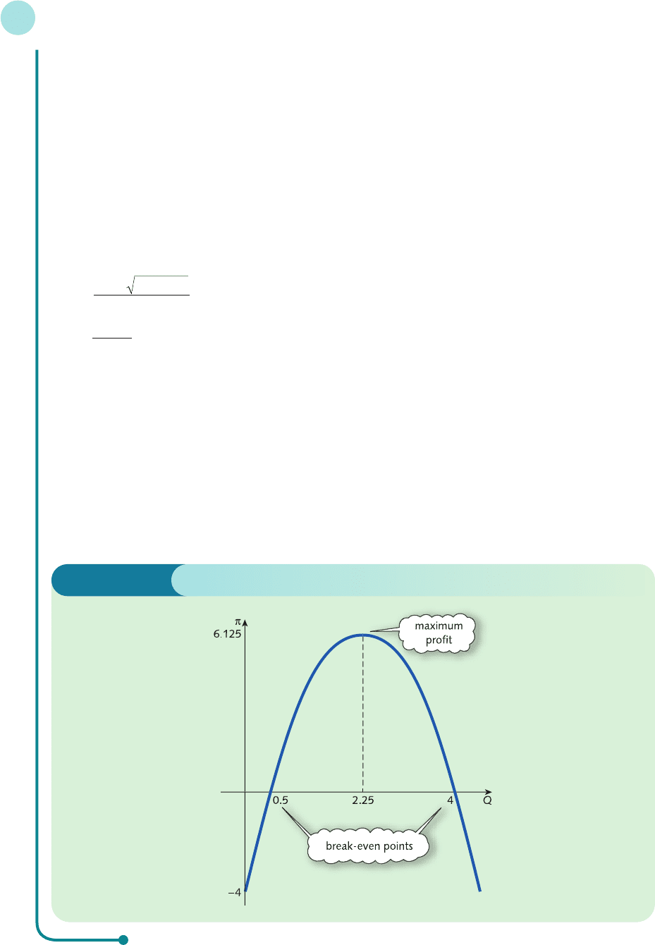
Step 1

The coefﬁcient of Q

is negative, so the graph has an inverted U shape.

Step 2

The constant term is −4, so the graph crosses the vertical axis when π=−4.

Step 3

The graph crosses the horizontal axis when π=0, so we need to solve the quadratic equation

−2Q

+ 9Q − 4 = 0

This can be done using ‘the formula’ to get

Q =

so Q = 0.5 and Q = 4.

The proﬁt curve is sketched in Figure 2.11.

(a) From Figure 2.11 we see that proﬁt is zero when Q = 0.5 and Q = 4.

(b) By symmetry, the parabola reaches its maximum halfway between 0.5 and 4: that is, at

Q =

/2(0.5 + 4) = 2.25

The corresponding proﬁt is given by

π=−2(2.25)

+ 9(2.25) − 4 = 6.125

−9 ± 7

−4

−± −

−

98132

( )

()

Non-linear Equations

136

Figure 2.11

MFE_C02b.qxd 16/12/2005 10:59 Page 136

2.2 • Revenue, cost and profit

137

Advice

It is important to notice the use of brackets in the previous derivation of π. A common stu-

dent mistake is to forget to include the brackets and just to write down

π=TR − TC

= 10Q − 2Q

− 4 + Q

=−2Q

+ 11Q − 4

This cannot be right, since the whole of the total cost needs to be subtracted from the total

revenue, not just the fixed costs. You might be surprised to learn that many economics

students make this sort of blunder, particularly under examination conditions. I hope that

if you have carefully worked through Section 1.4 on algebraic manipulation then you will

not fall into this category!

Practice Problem

3 If fixed costs are 25, variable costs per unit are 2 and the demand function is

P = 20 − Q

obtain an expression for π in terms of Q and hence sketch its graph.

(a) Find the levels of output which give a profit of 31.

(b) Find the maximum profit and the value of Q at which it is achieved.

Example

A ﬁrm’s proﬁt function is given by

π=−Q

+ 21Q − 18

Draw a graph of π against Q, over the range 0 ≤ Q ≤ 5, and hence estimate

(a) the interval in which π≥0

(b) the maximum proﬁt

Solution

Figure 2.12 (overleaf) shows the tabulated values of Q which have been entered in cells A4 to A8. In the

second column, cell B4 contains the formula to work out the corresponding values of π:

=−(A4)^3+21*A4 −18

This has been replicated down the proﬁt column by clicking and dragging in the usual way.

It can be seen that the maximum proﬁt occurs somewhere between 2 and 4, so it makes sense to add a

few extra entries in here so that the graph can be plotted more accurately in this region.

EXCEL



MFE_C02b.qxd 16/12/2005 10:59 Page 137

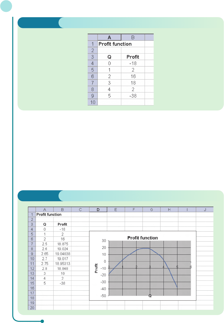
Initially, inserting extra rows for Q = 2.5 and 3.5 shows that the maximum occurs between 2.5 and 3.

Inserting a few more rows enables us to pinpoint the maximum proﬁt value more accurately, as shown in

Figure 2.13. At this stage, we can be conﬁdent that the maximum proﬁt occurs between Q = 2.6 and Q = 2.7.

The graph of the ﬁrm’s proﬁt function based on this table of values can now be drawn using Chart Wizard,

as shown in Figure 2.13.

This diagram shows that

(a) the ﬁrm makes a proﬁt for values of Q between 0.9 and 4.1

(b) the maximum proﬁt is about 19.

Non-linear Equations

138

Figure 2.12

Figure 2.13

MFE_C02b.qxd 16/12/2005 10:59 Page 138

2.2 • Revenue, cost and profit

139

Practice Problems

4 Given the following demand functions, express TR as a function of Q and hence sketch the graphs of

TR against Q.

(a)

P = 4 (b) P = 7/Q (c) P = 10 − 4Q

5 Given the following total revenue functions, find the corresponding demand functions

(a)

TR = 50Q − 4Q

(b) TR = 10

6 Given that fixed costs are 500 and that variable costs are 10 per unit, express TC and AC as functions

of Q. Hence sketch their graphs.

7 Given that fixed costs are 1 and that variable costs are Q + 1 per unit, express TC and AC as func-

tions of Q. Hence sketch their graphs.

8 Find an expression for the profit function given the demand function

2Q + P = 25

and the average cost function

AC =+5

Find the values of Q for which the firm

(a) breaks even

(b) makes a loss of 432 units

9 Sketch, on the same diagram, graphs of the total revenue and total cost functions,

TR =−2Q

+ 14Q

TC = 2Q + 10



Average cost Total cost per unit of output: AC = TC/Q.

Fixed costs Total costs that are independent of output.

L-shaped curve A term used by economists to describe the graph of a function, such as

f(x) = a + , which bends roughly like the letter L.

Proﬁt Total revenue minus total cost:

= TR − TC.

Rectangular hyperbola A term used by mathematicians to describe the graph of a func-

tion, such as f(x) = a + , which is a hyperbola with horizontal and vertical asymptotes.

Total cost The sum of the total variable and ﬁxed costs: TC = TVC + FC.

Total revenue A ﬁrm’s total earnings from the sales of a good: TR = PQ.

Variable costs Total costs that change according to the amount of output produced.

Key Terms

MFE_C02b.qxd 16/12/2005 10:59 Page 139