Jackson M.J. Micro and Nanomanufacturing

Meso-micromachining 161

1000

« 500

•^Ji^^

1 1

..._L

ri^

Compressive stress-strain curves

1 1

1 11

..-Li—

1.0

2.0

3.0 4.0 5.0

True strain e

(a)

6.0

7,0

8.0

1 2 3

True strain e

(b)

\ 40

I 30

i 20

, i 1

1,1...

j___

1 1 1 1 i 1 i

400

6.00 0.10 0.20 0.30 0.40 0.50 0.50 0.70 0.80 0.90 1.00 1.10 1.20 1.30 1.40

Logarithmic strain

(c)

(e)

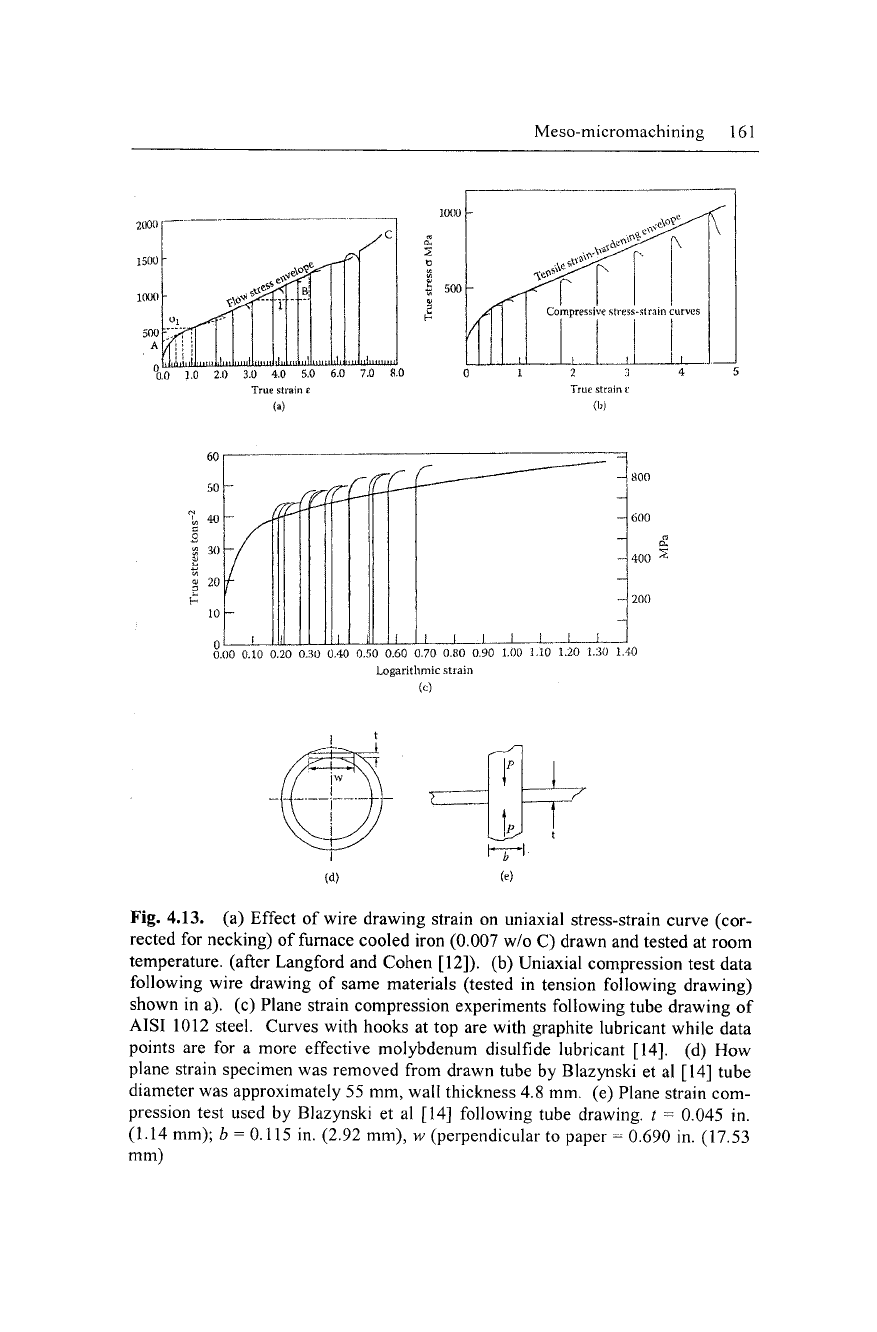
Fig. 4.13. (a) Effect of wire drawing strain on uniaxial stress-strain curve (cor-

rected for necking) of furnace cooled iron (0.007 w/o C) drawn and tested at room

temperature, (after Langford and Cohen [12]). (b) Uniaxial compression test data

following wire drawing of same materials (tested in tension following drawing)

shown in a), (c) Plane strain compression experiments following tube drawing of

AISI 1012 steel. Curves with hooks at top are with graphite lubricant while data

points are for a more effective molybdenum disulfide lubricant [14]. (d) How

plane strain specimen was removed from drawn tube by Blazynski et al [14] tube

diameter was approximately 55 mm, wall thickness 4.8 mm. (e) Plane strain com-

pression test used by Blazynski et al [14] following tube drawing, t = 0.045 in.

(1.14 mm); b = 0.115 in. (2.92 mm), w (perpendicular to paper - 0.690 in. (17.53

mm)

162 Micro-and Nanomanufacturing

1000

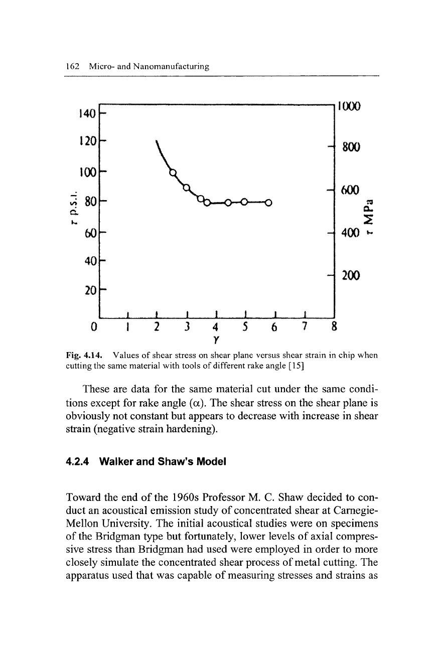
Fig. 4.14. Values of shear stress on shear plane versus shear strain in chip when

cutting the same material with tools of different rake angle [15]

These are data for the same material cut under the same condi-

tions except for rake angle (a). The shear stress on the shear plane is

obviously not constant but appears to decrease with increase in shear

strain (negative strain hardening).

4.2.4 Walker and Shaw's Model

Toward the end of

the

1960s Professor M. C. Shaw decided to con-

duct an acoustical emission study of concentrated shear at Carnegie-

Mellon University. The initial acoustical studies were on specimens

the

Bridgman type but fortunately, lower levels of axial compres-

sive stress than Bridgman had used were employed in order to more

closely simulate the concentrated shear process of metal cutting. The

apparatus used that was capable of measuring stresses and strains as

Meso-micromachining 163

well as acoustic signals arising from plastic flow is described in the

dissertation of T. J. Walker [16]. Two important results were ob-

tained:

A region of rather intense acoustical activity occurred at

the yield point followed by a quieter region until a shear strain of

about 1.5 was reached. At this point there was a rather abrupt in-

crease in acoustical activity that continued to the strain at fracture

which was appreciably greater than 1.5.

The shear stress appeared to reach a maximum at strain

corresponding to the beginning of the second acoustical activity (y -

1.5)

The presence of the notches in the Bridgman specimen (Fig.

4.12) made interpretation of stress-strain results somewhat uncertain.

Therefore, a new specimen was designed (Fig. 4.15) which substi-

tutes simple shear for torsion with normal stress on the shear plane.

By empirically adjusting distance Ax (Fig. 4.15) to a value of 0.25

mm it was possible to confine all the plastic shear strain to the re-

duced area, thus making it possible to readily determine the shear

strain (y ^Ay/

Ax).

When the width of minimum section was greater

or less than 0.25 mm, the extent of plastic strain observed in a trans-

verse micrograph at the minimum section either did not extend com-

pletely across the 0.25 mm dimension or beyond this width.

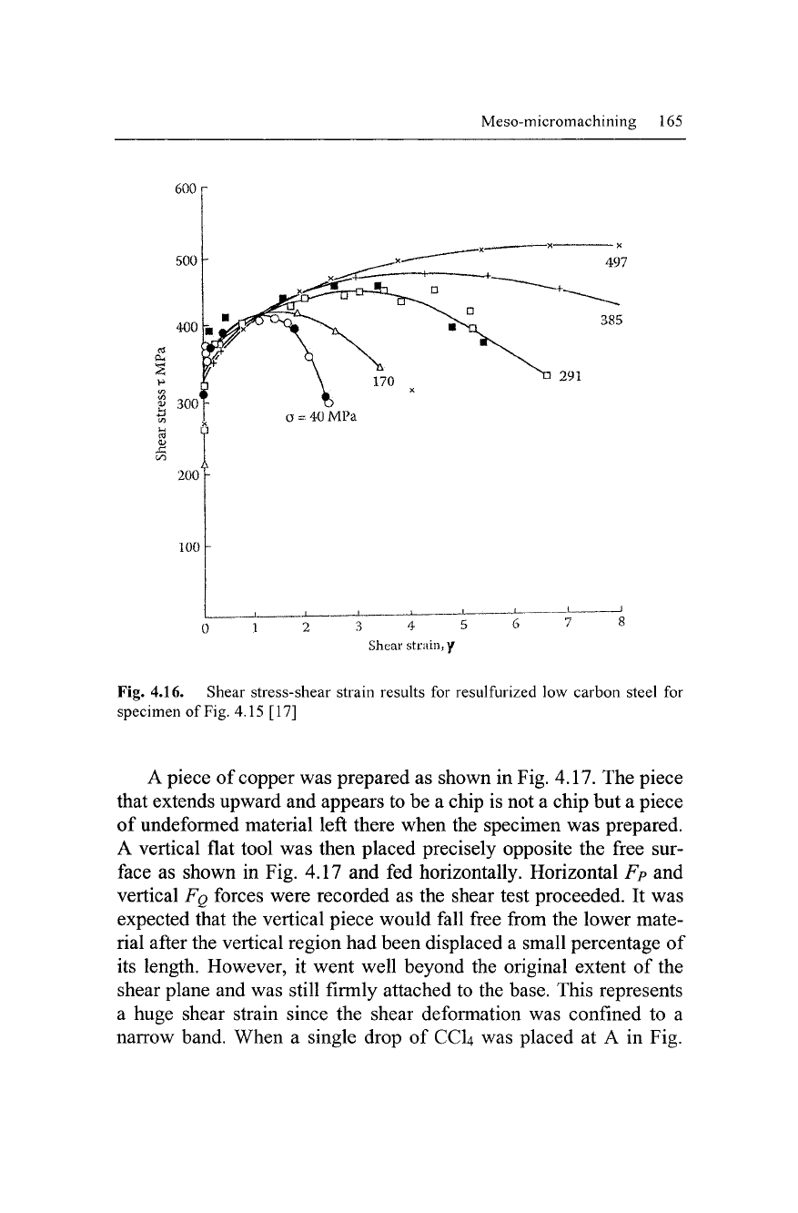
A representative set of curves is shown in Fig. 4.16 for re-

sulfurised low carbon steel. Similar results were obtained for non-

resulfurised steels and other ductile metals. There is little difference

in the curves for different values of normal stress on the shear plane

(a) to a shear strain of about 1.5.

This is in agreement with Bridgman. However, beyond this

strain the curves differ substantially with compressive stress on the

shear plane. At large strains

(T)

was found to decrease with increase

in (y), a result that does not agree with Bridgman [11]. When the re-

sults of Fig. 4.13a and 4.16 are compared they are seen to be very

different. In the case of Fig. 4.13a strain hardening is positive to

normal strains as high as 7. In the case of

Fig.

4.16 strain hardening

becomes negative above a particular shear strain that increases with

normal stress on the shear plane.

164 Micro-and Nanomanufacturing

Fig. 4.15. Plane strain simple shear-compression specimen of Walker and Shaw

[17]

From Fig. 4.16 it is seen that for a low value of normal stress on

the shear plane of 40 MPa strain hardening appears to be negative at

a shear strain of about 1.5; that is, when the normal stress on the

shear plane is about 10% of the maximum shear stress reached,

negative strain hardening sets in at a shear strain of about 1.5. On the

other hand, strain hardening remains positive to a normal strain of

about 8 when the normal stress on the shear plane is about equal to

the maximum shear stress (note curve for a = 497 MPa in Fig. 4.16).

4.2.5 Usui's Model

In Usui et al [18] an experiment is described designed to determine

why CCI4 is such an effective cutting fluid at low cutting speeds.

Since this also has a bearing on the role of microcracks in large

strain deformation, it is considered here.

Meso-micromachining 165

600T

497

385

g 300

200'

100

G==40MPa

•--1 1—-

3 4 5

Shear strain, y

Fig. 4.16. Shear stress-shear strain results for resulfurized low carbon steel for

specimen of

Fig.

4.15 [17]

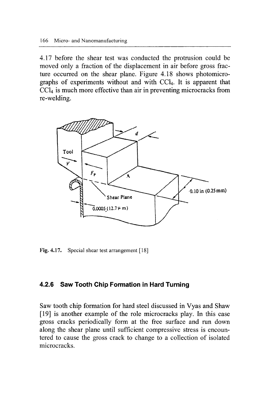
A piece of copper was prepared as shown in Fig. 4.17. The piece

that extends upward and appears to be a chip is not a chip but a piece

of undeformed material left there when the specimen was prepared.

A vertical flat tool was then placed precisely opposite the free sur-

face as shown in Fig. 4.17 and fed horizontally. Horizontal Fp and

vertical FQ forces were recorded as the shear test proceeded. It was

expected that the vertical piece would fall free from the lower mate-

rial after the vertical region had been displaced a small percentage of

its length. However, it went well beyond the original extent of the

shear plane and was still firmly attached to the base. This represents

a huge shear strain since the shear deformation was confined to a

narrow band. When a single drop of CCI4 was placed at A in Fig.

166 Micro-and Nanomanufacturing

4.17 before the shear test was conducted the protrusion could be

moved only a fraction of the displacement in air before gross frac-

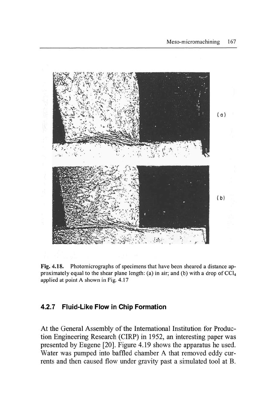
ture occurred on the shear plane. Figure 4.18 shows photomicro-

graphs of experiments without and with CCI4. It is apparent that

CCI4 is much more effective than air in preventing microcracks from

re-welding.

O.IO

in (0.25 mm)

Fig. 4.17. Special shear test arrangement [18]

4.2.6 Saw Tooth Chip Formation in Hard Turning

Saw tooth chip formation for hard steel discussed in Vyas and Shaw

[19] is another example of the role microcracks play. In this case

gross cracks periodically form at the free surface and run down

along the shear plane until sufficient compressive stress is encoun-

tered to cause the gross crack to change to a collection of isolated

microcracks.

Meso-micromachining 167

(Q)

Fig. 4.18. Photomicrographs of specimens that have been sheared a distance ap-

proximately equal to the shear plane length: (a) in air; and (b) with a drop of CCI4

applied at point A shown in Fig. 4.17

4.2.7 Fluid-Like Flow in Chip Formation

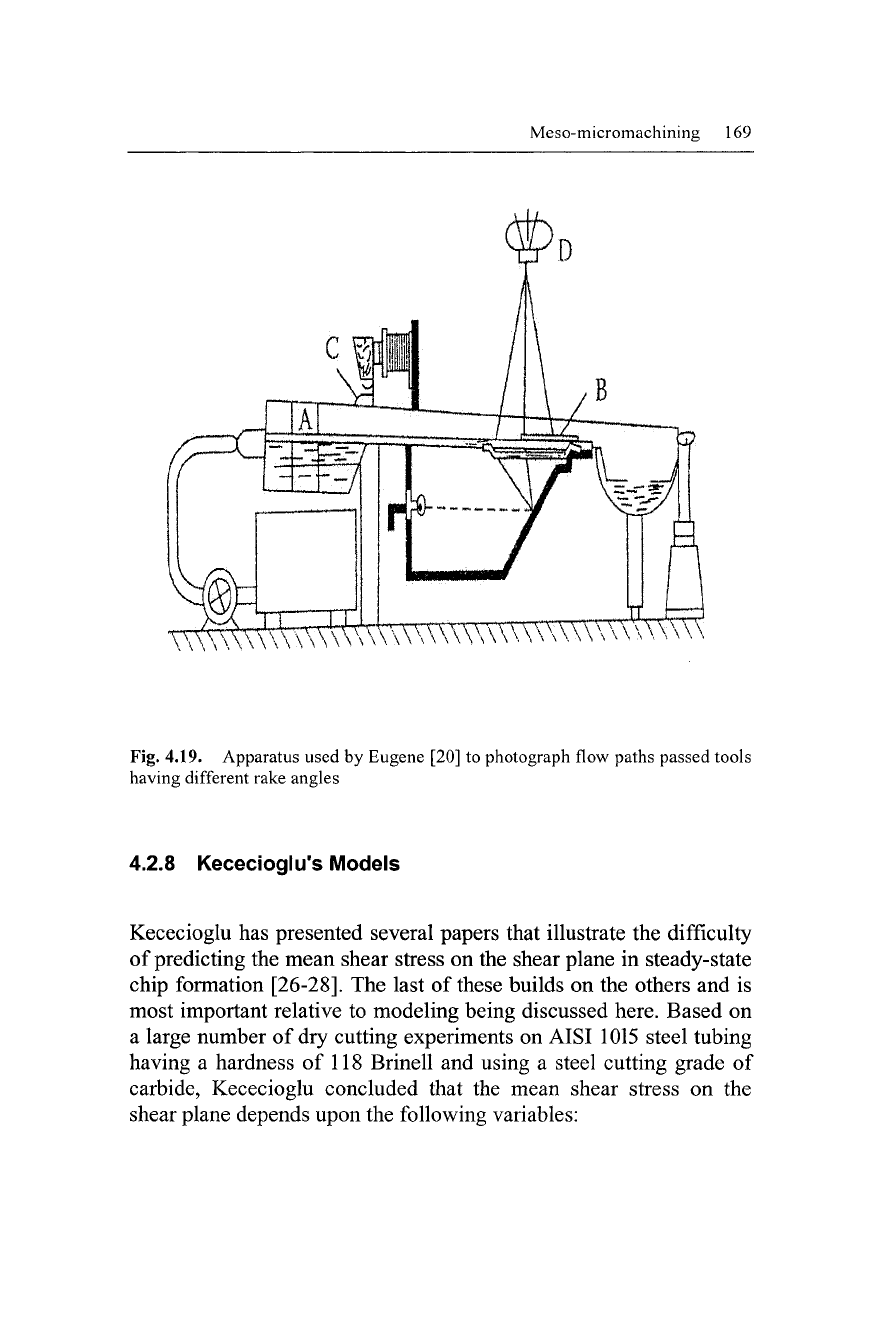
At the General Assembly of the International Institution for Produc-

tion Engineering Research (CIRP) in 1952, an interesting paper was

presented by Eugene [20]. Figure 4.19 shows the apparatus he used.

Water was pumped into baffled chamber A that removed eddy cur-

rents and then caused flow under gravity past a simulated tool at B.

168 Micro-and Nanomanufacturing

Powdered bakelite was introduced at C to make the streamlines visi-

ble as the fluid flowed past the tool. The photographs taken by the

camera at D were remarkably similar to quick stop photomicro-

graphs of actual chips. It was thought by this author at the time that

any similarity between fluid flow and plastic flow of a solid was not

to be expected. That was long before it was clear that the only logi-

cal explanation for the results of Bridgman and Merchant involve

microfracture [21].

At the General Assembly of CIRP 47 years later, a paper was

presented that again suggests that metal cutting might be modeled by

a fluid [22]. However, this paper was concerned with ultraprecision

machining (depths of cut < 4 \xm) and potential flow analysis was

employed instead of the experimental approach taken by Eugene.

It is interesting to note that chemists relate the flow of liquids to

the migration of vacancies (voids) just as physicists relate ordinary

plastic flow of solid metals to the migration of dislocations. Henry

Eyring and co-workers [24-26] have studied the marked changes in

volume, entropy and fluidity that occur when a solid melts. For ex-

ample, a 12% increase in volume accompanies melting of Argon,

suggesting the removal of every eighth molecule as a vacancy upon

melting. This is consistent with X-ray diffraction of liquid argon that

showed good short-range order but poor long-range order. The rela-

tive ease of diffusion of these vacancies accounts for the increased

fluidity that accompanies melting. A random distribution of vacan-

cies is also consistent with the increase in entropy observed on melt-

ing. Eyring's theory of fluid flow was initially termed the "hole the-

ory of fluid flow" but later "The Significant Structure Theory" which

is the title of the Eyring-Jhon book [25].

According to this theory the vacancies in a liquid move through

a sea of molecules. Eyring's theory of liquid flow is mentioned here

since it explains why the flow of a liquid approximates the flow of

metal passed a tool in chip formation. In this case microcracks

(voids) move through a sea of crystalline solid.

Meso-micromachining 1(

TWAVA

KWV^\\VV^^V^^\^'^V\\\\\\\\\\^AU

Fig. 4.19. Apparatus used by Eugene [20] to photograph flow paths passed tools

having different rake angles

4.2.8 Kececioglu's Models

Kececioglu has presented several papers that illustrate the difficulty

of predicting the mean shear stress on the shear plane in steady-state

chip formation [26-28]. The last of these builds on the others and is

most important relative to modeling being discussed here. Based on

a large number of dry cutting experiments on AISI 1015 steel tubing

having a hardness of 118 Brinell and using a steel cutting grade of

carbide, Kececioglu concluded that the mean shear stress on the

shear plane depends upon the following variables:

170 Micro-and Nanomanufacturing

mean normal stress on the shear plane

(GS)

the shear volume of the shear zone (e)

the mean strain rate in the shear plane (y)

the mean temperature of the shear plane (0$)

the degree of strain hardening in the work before cut-

ting

If this were not complicated enough it is clear from Kececioglu's

experimental results that these items do not act independently (i.e.,

the influence of a high normal stress on the shear plane on shear

stress on the shear plane depends upon the combination of other

variables pertaining). This is an important result since it means that

in general it is not possible to extrapolate materials test values of

shear stress to vastly different cutting conditions.

It is interesting to note that Kececioglu suggests that the specific

energy should be related to the shear plane area (e) instead of (t) as

in most treatments of metal cutting mechanics. The shear plane area

= Z?(t/sin(t))

(in^

or mm^) (4.14)

This appears to be a useful suggestion. In both cases the inverse

relation between u and

or e is due to the greater chance of encoun-

tering a stress-reducing defect as ^ or e increases. The use of e in-

stead of Hs a more general although more complex way of express-

ing the "size effect". The range of values covered by Kececioglu in

his orthogonal experiments on AISI 1015 steel were as follows:

rake angle: -10 to +37 degrees

undeformed chip thickness (0: 0.004 to 0.012 in (0.2 to 0.3

mm)

cutting speed (V): 1 26 to 746 fpm (38.4 to 227.4 m/min)

inclination angle (/): 0 to 35 degrees

This resulted in the following wide range of dependent variables:

width of shear zone : 0.002 to 0.007 inch (0.10 to 0.18 mm)

Jackson M.J. Micro and Nanomanufacturing

Подождите немного. Документ загружается.