Hirsch M., Smale S., Devaney R., Differential Equations, Dynamical Systems, and an Introduction to Chaos
Подождите немного. Документ загружается.


296 Chapter 13 Applications in Mechanics
To fully understand the flow on , we introduce the angular variable ψ in
each u
r
u
θ
–plane via
u
r
=
√
2sinψ
u
θ
=
√
2cosψ.
The torus is now parameterized by θ and ψ.Inθψ coordinates, the system
becomes
˙
θ =
√
2cosψ
˙
ψ =
1
√
2
cosψ.
The circles C
±
are now given by ψ =±π/2. Eliminating time from this
equation, we find
dψ
dθ
=
1
2
.
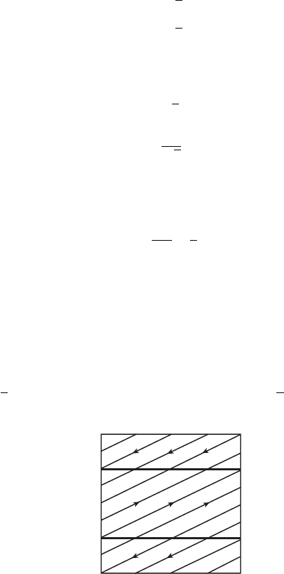
Thus all nonequilibrium solutions have constant slope 1/2 when viewed in θψ
coordinates. See Figure 13.4.
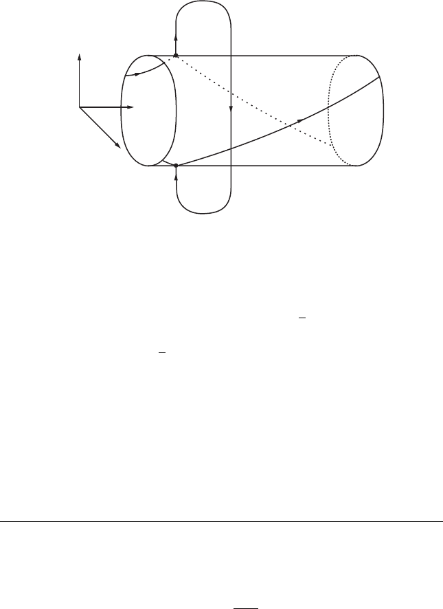
Now recall the collision-ejection solutions described in Section 13.4. Each
of these solutions leaves the origin and then returns along a ray θ =θ
∗
in con-
figuration space. The solution departs with v
r
> 0 (and so u
r
> 0) and returns
with v
r
< 0(u
r
< 0). In our new four-dimensional coordinate system, it follows
that this solution forms an unstable curve associated to the equilibrium point
(0,θ
∗
,
√
2,0) and a stable curve associated to (0,θ
∗
,−
√
2,0). See Figure 13.5.
C
⫹
C
⫺
v
h
Figure 13.4 Solutions on
in θψ coordinates. Recall that
θ and ψ are both defined
mod 2π , so opposite sides of
this square are identified to
form a torus.

13.8 Exploration: Other Central Force Problems 297
D
h
u
h
u
r
h
∗
Figure 13.5 A collision-ejection solution in the region
r > 0 leaving and returning to and a connecting orbit
on the collision surface.
What happens to nearby noncollision solutions? Well, they come close to
the “lower” equilibrium point with θ =θ
∗
,u
r
=−
√
2, then follow one of two
branches of the unstable curve through this point up to the “upper” equilib-
rium point θ =θ
∗
,u
r
=+
√
2, and then depart near the unstable curve leaving
this equilibrium point. Interpreting this motion in configuration space, we see
that each near-collision solution approaches the origin and then retreats after
θ either increases or decreases by 2π units. Of course, we know this already,
since these solutions whip around the origin in tight ellipses.
13.8 Exploration: Other Central Force
Problems
In this exploration, we consider the (non-Newtonian) central force problem
for which the potential energy is given by
U (X ) =
1
|X|
ν
where ν > 1. The primary goal is to understand near-collision solutions.
1. Write this system in polar coordinates (r,θ,v
r
,v
θ
) and state explicitly the
formulas for total energy and angular momentum.
2. Using a computer, investigate the behavior of solutions of this system
when h<0 and =0.

298 Chapter 13 Applications in Mechanics
3. Blow up the singularity at the origin via the change of variables
u
r
=r
ν/2
v
r
, u
θ
=r
ν/2
v
θ
and an appropriate change of timescale and write down the new system.
4. Compute the vector field on the collision surface determined in r =0
by the total energy relation.
5. Describe the bifurcation that occurs on when ν =2.
6. Describe the structure of
h,
for all ν > 1.
7. Describe the change of structure of
h,
that occurs when ν passes
through the value 2.
8. Describe the behavior of solutions in
h,
when ν > 2.
9. Suppose 1 < ν < 2. Describe the behavior of solutions as they pass close
to the singularity at the origin.
10. Using the fact that solutions of this system are preserved by rotations
about the origin, describe the behavior of solutions in
h,
when h<0
and =0.
13.9 Exploration: Classical Limits of
Quantum Mechanical Systems
In this exploration we investigate the anisotropic Kepler problem. This is a
classical mechanical system with two degrees of freedom that depends on a
parameter μ. When μ =1 the system reduces to the Newtonian central force
system discussed in Section 13.4. When μ > 1 some anisotropy is introduced
into the system, so that we no longer have a central force field. We still have
some collision-ejection orbits, as in the central force system, but the behavior
of nearby orbits is quite different from those when μ =1.
The anisotropic Kepler problem was first introduced by Gutzwiller as a
classical mechanical approximation to certain quantum mechanical systems.
In particular, this system arises naturally when one looks for bound states of an
electron near a donor impurity of a semiconductor. Here the potential is due
to an ordinary Coulomb field, while the kinetic energy becomes anisotropic
because of the electronic band structure in the solid. Equivalently, we can view
this system as having an anisotropic potential energy function. Gutzwiller
suggests that this situation is akin to an electron whose mass in one direction
is larger than in other directions. For more background on the quantum
mechanical applications of this work, refer to [22].
The anisotropic Kepler system is given by
x
=
−μx
(μx
2
+y
2
)
3/2

Exercises 299
y
=
−y
(μx
2
+y
2
)
3/2
where μ is a parameter that we assume is greater than 1.
1. Show that this system is conservative with potential energy given by
U (x,y) =
−1
μx
2
+y
2
and write down an explicit formula for total energy.
2. Describe the geometry of the energy surface
h
for energy h<0.
3. Restricting to the case of negative energy, show that the only solutions
that meet the zero velocity curve and are straight-line collision-ejection
orbits for the system lie on the x- and y-axes in configuration space.
4. Show that angular momentum is no longer an integral for this system.
5. Rewrite this system in polar coordinates.
6. Using a change of variables and time rescaling as for the Newtonian
central force problem (Section 13.7), blow up the singularity and write
down a new system without any singularities at r =0.
7. Describe the structure of the collision surface (the intersection of
h
with r =0 in the scaled coordinates). In particular, why would someone
call this surface a “bumpy torus?”
8. Find all equilibrium points on and determine the eigenvalues of the
linearized system at these points. Determine which equilibria on are
sinks, sources, and saddles.
9. Explain the bifurcation that occurs on when μ =9/8.
10. Find a function that is nondecreasing along all nonequilibrium solutions
in .
11. Determine the fate of the stable and unstable curves of the saddle points
in the collision surface. Hint: Rewrite the equation on this surface to
eliminate time and estimate the slope of solutions as they climb up .
12. When μ >9/8, describe in qualitative terms what happens to solutions
that approach collision close to the collision-ejection orbits on the x-axis.
In particular, how do they retreat from the origin in the configuration
space? How do solutions approach collision when traveling near the
y-axis?
EXERCISES
1. Which of the following force fields on R
2
are conservative?
(a) F(x, y) =(−x
2
, −2y
2
)

300 Chapter 13 Applications in Mechanics
(b) F(x, y) =(x
2
−y
2
,2xy)
(c) F(x, y) =(x,0)
2. Prove that the equation
1
r
=
1
h
(1+ cos θ)
determines a hyperbola, parabola, and ellipse when > 1, =1, and
< 1, respectively.
3. Consider the case of a particle moving directly away from the origin at
time t =0 in the Newtonian central force system. Find a specific formula
for this solution and discuss the corresponding motion of the particle. For
which initial conditions does the particle eventually reverse direction?
4. In the Newtonian central force system, describe the geometry of
h,
when h>0 and h =0.
5. Let F(X ) be a force field on
R
3
. Let X
0
, X
1
be points in R
3
and let Y (s)
be a path in
R
3
with s
0
≤s ≤s
1
, parametrized by arc length s, from X
0
to
X
1
. The work done in moving a particle along this path is defined to be
the integral
s
1
s
0
F(y(s))·y
(s)ds
where Y
(s) is the (unit) tangent vector to the path. Prove that the force
field is conservative if and only if the work is independent of the path. In
fact, if F =−grad V , then the work done is V (X
1
)−V (X
0
).
6. Describe solutions to the non-Newtonian central force system given by
X
=−
X
|X|
4
.
7. Discuss solutions of the equation
X
=
X
|X|
3
.
This equation corresponds to a repulsive rather than attractive force at
the origin.
8. This and the next two problems deal with the two-body problem. Let the
potential energy be
U =
gm
1
m
2
|X
2
−X
1
|

Exercises 301
and
grad
j
(U ) =
∂U
∂x
j
1
,
∂U
∂x
j
2
,
∂U
∂x
j
3
.
Show that the equations for the two-body problem can be written
m
j
X
j
=−grad
j
(U ).
9. Show that the total energy K +U of the system is a constant of the motion,
where
K =
1
2
m
1
|V
1
|
2
+m
2
|V
2
|
2
.
10. Define the angular momentum of the system by
=m
1
(X
1
×V
1
)+m
2
(X
2
×V
2
)
and show that is also a first integral.
This Page Intentionally Left Blank

14
The Lorenz System
So far, in all of the differential equations we have studied, we have not encoun-
tered any “chaos.” The reason is simple: The linear systems of the first few
chapters always exhibit straightforward, predictable behavior. (OK, we may
see solutions wrap densely around a torus as in the oscillators of Chapter 6, but
this is not chaos.) Also, for the nonlinear planar systems of the last few chap-
ters, the Poincaré-Bendixson theorem completely eliminates any possibility of
chaotic behavior. So, to find chaotic behavior, we need to look at nonlinear,
higher dimensional systems.
In this chapter we investigate the system that is, without doubt, the most
famous of all chaotic differential equations, the Lorenz system from meteo-
rology. First formulated in 1963 by E. N. Lorenz as a vastly oversimplified
model of atmospheric convection, this system possesses what has come to
be known as a “strange attractor.” Before the Lorenz model started making
headlines, the only types of stable attractors known in differential equations
were equilibria and closed orbits. The Lorenz system truly opened up new
horizons in all areas of science and engineering, because many of the phe-
nomena present in the Lorenz system have later been found in all of the
areas we have previously investigated (biology, circuit theory, mechanics, and
elsewhere).
In the ensuing 40 years, much progress has been made in the study of
chaotic systems. Be forewarned, however, that the analysis of the chaotic
behavior of particular systems like the Lorenz system is usually extremely
difficult. Most of the chaotic behavior that is readily understandable arises
from geometric models for particular differential equations, rather than from
303

304 Chapter 14 The Lorenz System
the actual equations themselves. Indeed, this is the avenue we pursue here. We
will present a geometric model for the Lorenz system that can be completely
analyzed using tools from discrete dynamics. Although this model has been
known for some 30 years, it is interesting to note the fact that this model was
only shown to be equivalent to the Lorenz system in the year 1999.
14.1 Introduction to the Lorenz System
In 1963, E. N. Lorenz [29] attempted to set up a system of differential equations
that would explain some of the unpredictable behavior of the weather. Most
viable models for weather involve partial differential equations; Lorenz sought
a much simpler and easier-to-analyze system.
The Lorenz model may be somewhat inaccurately thought of as follows.
Imagine a planet whose “atmosphere” consists of a single fluid particle. As on
earth, this particle is heated from below (and hence rises) and cooled from
above (so then falls back down). Can a weather expert predict the “weather”
on this planet? Sadly, the answer is no, which raises a lot of questions about
the possibility of accurate weather prediction down here on earth, where we
have quite a few more particles in our atmosphere.
A little more precisely, Lorenz looked at a two-dimensional fluid cell that
was heated from below and cooled from above. The fluid motion can be
described by a system of differential equations involving infinitely many vari-
ables. Lorenz made the tremendous simplifying assumption that all but three
of these variables remained constant. The remaining independent variables
then measured, roughly speaking, the rate of convective “overturning” (x),
and the horizontal and vertical temperature variation (y and z, respectively).
The resulting motion led to a three-dimensional system of differential equa-
tions that involved three parameters: the Prandtl number σ , the Rayleigh
number r, and another parameter b that is related to the physical size of the
system. When all of these simplifications were made, the system of differential
equations involved only two nonlinear terms and was given by
x
= σ (y − x)
y
= rx − y − xz
z
= xy − bz.
In this system all three parameters are assumed to be positive and, moreover,
σ >b+ 1. We denote this system by X
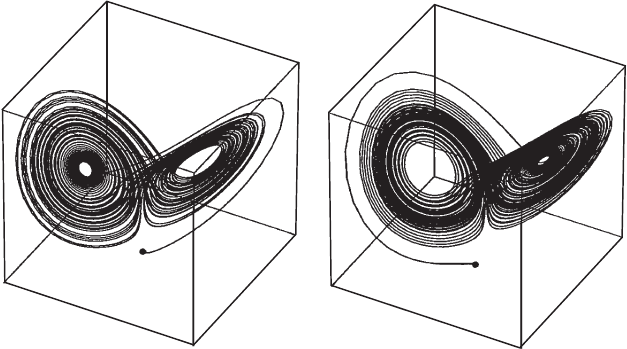
= L(X). In Figure 14.1, we have
displayed the solution curves through two different initial conditions P
1
=
(0, 2, 0) and P
2
= (0, −2, 0) when the parameters are σ = 10, b = 8/3, and

14.1 Introduction to the Lorenz System 305
x
y
z
P
1
P
2
Figure 14.1 The Lorenz attractor. Two solutions with initial conditions P
1
=
(0, 2, 0) and P
2
= (0, −2, 0).
r = 28. These are the original parameters that led to Lorenz’s discovery. Note
how both solutions start out very differently, but eventually have more or less
the same fate: They both seem to wind around a pair of points, alternating at
times which point they encircle. This is the first important fact about the Lorenz
system: All nonequilibrium solutions tend eventually to the same complicated
set, the so-called Lorenz attractor.
There is another important ingredient lurking in the background here. In
Figure 14.1, we started with two relatively far apart initial conditions. Had we
started with two very close initial conditions, we would not have observed the
“transient behavior” apparent in Figure 14.1. Rather, more or less the same
picture would have resulted for each solution. This, however, is misleading.
When we plot the actual coordinates of the solutions, we see that these two
solutions actually move quite far apart during their journey around the Lorenz
attractor. This is illustrated in Figure 14.2, where we have graphed the x
coordinates of two solutions that start out nearby, one at (0, 2, 0), the other (in
gray) at (0, 2. 01, 0). These graphs are nearly identical for a certain time period,
but then they differ considerably as one solution travels around one of the lobes
of the attractor while the other solution travels around the other. No matter
how close two solutions start, they always move apart in this manner when
they are close to the attractor. This is sensitive dependence on initial conditions,
one of the main features of a chaotic system.
We will describe in detail the concept of an attractor and chaos in this
chapter. But first, we need to investigate some of the more familiar features of
the system.
