Hillert M. Phase Equilibria, Phase Diagrams and Phase Transformations: Their Thermodynamic Basis

Подождите немного. Документ загружается.

10.7 Selection of axes in mixed diagrams 225

1500

1000

500

0 0.2 0.4 0.6

fcc

bcc

T (K)

Figure 10.23 T , x

diagram for Fe–Cr–C at 1 bar and a

= 0.3. This is not a true phase diagram.

1.02 1.06

H (kJ/mol Fe)

fcc

cem

fcc

(a) (b)

Figure 10.24 H

, a

diagram for Fe–C at 1 bar. This is not a true phase diagram as revealed by

the overlapping two-phase ﬁelds, shown when the tie-lines are included in (b).

conjugate variables. That is revealed by the tie-lines which are included in Fig. 10.24(b).

The reason is that the numerical values used for H

refer to reference states of Fe and

Cat298Kbuta

refers to graphite at the actual temperatures. It is evident that one

should also be careful when representing the oxygen potential with P

.Itisonly under

isothermal conditions that it should be combined with an axis for a molar quantity given

relative to references at 298 K. It should be noted that the diagrams in Figs 8.13 and

8.14 used µ

−

or (µ

−

)/T as an axis and

was deﬁned at the actual

temperature which varied. That did not cause any problem because there was no molar

axis in those diagrams.

Exercise 10.10

Figure 10.23 showed an incorrect selection of axes. If one really wanted to section at a

constant value of a

,what composition axis should one have used?

226 Projected and mixed phase diagrams

Hint

Consult the Tables 9.1, 9.2 and 9.3.

Solution

represents µ

/T which may be combined with −1/ T , −P, and z

(according to

ﬁfth row in Table 9.2)oru

(according to ﬁfth row in Table 9.3). Of course, −1/T could

be replaced by T.

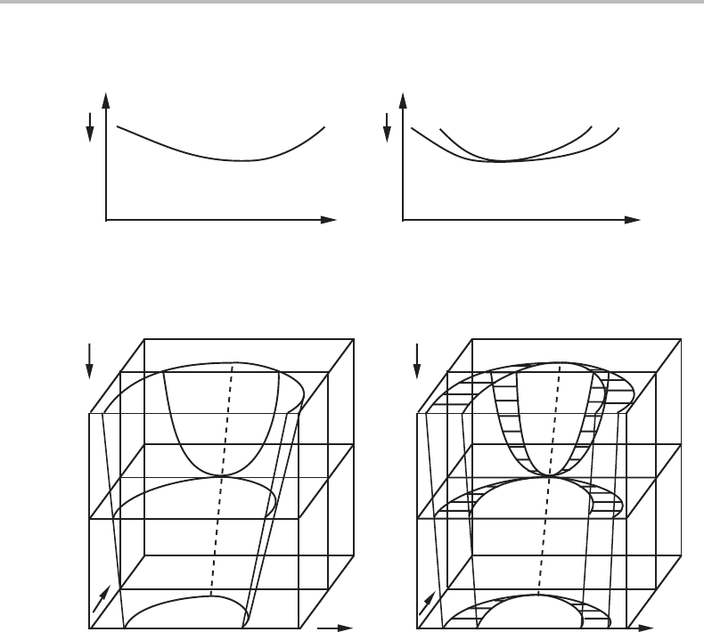
10.8 Konovalov’s rule

The rule that two one-phase ﬁelds are separated from each other by a positive distance,

when the proper molar quantity is introduced instead of a potential, was described in

Section 9.1. That rule is not as trivial as it may appear. It was discovered experimentally

by Konovalov [20]when measuring the vapour pressure of liquid solutions of water and

various organic substances under isothermal conditions. He established that, compared

with the solution, the vapour contains a higher relative content of that component which,

when added to the solution, increases the total vapour pressure. In addition, he found

two cases with a pressure maximum and realized that the liquid and vapour must have

the same composition at such a point. A case of this type is shown in Fig. 10.25, and it

is evident that it is simply due to the fact that the molar quantity which is used, here z

replaces a potential whose axis happens to be parallel to a line tangential to the linear two-

phase ﬁeld in the potential diagram. Except for that, the system has no unique properties

at this point. The point is sometimes called a singular point and the equilibrium under

this special condition is called singular equilibrium.

Figure 10.26(a) shows a three-dimensional diagram for the same kind of system but

including both temperature and pressure axes. It was presented in Fig. 8.23 and it was

then concluded that an extremum in P at constant T must lead to an extremum in T at

constant P. The corresponding diagram, where z

has been introduced instead of µ

,is

shown in Fig. 10.26(b) and it conﬁrms that the two phases have the same composition at

the point of extremum considered. In fact, there is a whole series of such points, marked

as a dotted line. This is the locus of points of tangency for tangents parallel to the µ

or z

axis. That line represents a singular equilibrium and could be included in the T, P

diagram, obtained by projecting in the µ

(i.e. z

) direction, Schreinemakers’ projection.

The line representing singular equilibrium is called a singular curve. Singular equilibria

will be further discussed in Sections 12.6 and 13.7 to 13.9.

A major difference between univariant lines and singular curves should be noted. A

univariant line shows exactly where a particular univariant equilibrium occurs. A singular

curve shows the maximum extension of a divariant equilibrium which is otherwise not

shown in the diagram. It would thus be wise to indicate on what side of a singular curve

the particular equilibrium exists. This is done in Fig. 10.27,which is a projection of

Fig. 10.26.

10.8 Konovalov’s rule 227

vapour

liquid liquid

(a) (b)

Figure 10.25 An isothermal section of a binary diagram with a singular point for two phases

illustrating Konovalov’s rule.

(a) (b)

Figure 10.26 (a) A two-phase equilibrium in a binary system illustrated with the complete

three-dimensional potential phase diagram. Points of tangency for lines parallel to the µ

axis

are marked with a dotted line. (b) After µ

has been replaced by its conjugate molar quantity,

, the phases still coincide along the dotted line where the two phases have the same

composition, expressed through z

Points of extremum in P and T were discussed in Section 8.9 and Konovalov’s rule was

actually derived there in an analytical way, using the ordinary molar quantities, S

, V

and x

.InChapter 8 and the present one we have mainly used molar quantities deﬁned by

dividing the integral quantities with the content of a certain component, N

for instance.

We denote these quantities with S

, V

and z

.However, if all the molar quantities we

are interested in are molar contents, then the results look the same in both notations. As

an example, the insertion of x

= x

in the result for p = c in Section 8.9 yields

0 =



1 x

..x



..x



1 z

..z



· x

...x

(10.10)

0 =



1 z

..z



. (10.11)

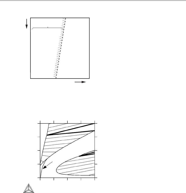
228 Projected and mixed phase diagrams

α+β

Figure 10.27 Singular curve showing the maximum extension of the α + β equilibrium in

Fig. 10.25. Projected in the z

direction. The α + β surface is folded and to the left of the curve

one would intersect that surface twice by moving in the projected direction, i.e., perpendicular

to the picture.

0 0.5 1.0 1.5 2.0

mass-% N

mass-% Cr

= 0.75

Figure 10.28 See Exercise 10.11.

We shall continue to use z

but it should be remembered that the results hold for x

well.

The importance of Konovalov’s rule stems from the fact that composition is often

used as an experimental variable. A system with a composition at a point of maximum

or minimum undergoes an azeotropic or congruent transformation on passing through

it and such a point is often given a special name, azeotropic (actually meaning ‘boiling

unchanged’) or congruent.

Exercise 10.11

The phase diagram (Fig. 10.28)isanisobarothermal section at 1273 K and 1 bar of the

Fe–Cr–N phase diagram under conditions where N

gas does not form. An isoactivity

10.9 General rule for singular equilibria 229

0.35

(a) (b)

0.30

0.25

0.20

0.15

0.10

0 0.04 0.08 0.50 0.75 1.00

= 0.75

Figure 10.29 Solution to Exercise 10.11.

line for N has been drawn in the γ phase ﬁeld. Show a reasonable continuation of it after

ﬁrst sketching the corresponding µ

, a

phase diagram.

Hint

Notice that there is a tie-line for which the α and γ phases have the same Cr content. It

should be a point of extremum for the N potential (or N activity).

Solution

The solution is given in Fig. 10.29.

10.9 General rule for singular equilibria

It is evident that Konovalov’s rule does not only apply to composition. It may thus be

generalized. Suppose that a linear two-phase ﬁeld in a Y

, Y

diagram, determined at

constant values of all the other potentials except Y

,which is chosen as the dependent

potential, shows a Y

maximum or minimum. At the point of extremum the two phases

must have the same value of X

m−1

. Furthermore, if Y

is kept constant and another

potential is allowed to vary, it will also have an extremum at the same value of X

m−1

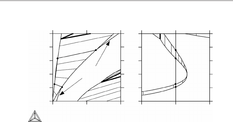
Let us now consider a two-phase equilibrium in an isobaric potential diagram for a

ternary system, which is three-dimensional. Thus, p = c − 1. Suppose there is a point

of tangency for a plane parallel to the µ

, µ

plane (i.e. an isothermal plane) as shown

in Fig. 10.30(a) which is a reproduction of Fig. 8.24.Asdemonstrated in Fig. 10.30(b),

the two phases thus have the same composition and the point of extremum is a congruent

transformation point. This was already proved in Section 8.9 using an analytical method.

230 Projected and mixed phase diagrams

Figure 10.30 (a) Isobaric potential phase diagram of a ternary system with a doubly singular

point on a divariant phase ﬁeld. Thin lines represent points of tangency for lines parallel to the

or µ

axis. Their intersection is a point of tangency on a µ

,µ

plane. It gives an extremum

of T. (b) By replacing µ

and µ

with their conjugate molar quantities, z

and z

,itisshown

that the two phases in the point of T extremum must have the same z

and the same z

value.

The point of extremum thus deﬁnes the composition of an alloy which can transform

congruently between the two phases.

The point of extremum in Fig. 10.30 may be characterized as a doubly singular point.

It would also appear in a diagram with a P axis under a constant value of T equal to the

extreme value. In order to show in one diagram that this point is an extremum for P as

well as T, one would need a fourth dimension. It is evident that the doubly singular point

in Fig. 10.30 would fall at a different T value if the constant P value was different and in

a P, T projection all such points would form a line, a doubly singular curve.

From Section 8.9 it is evident that Konovalov’s rule is just a special case of a more

general rule. In fact, for the ternary case, p = c = 3, it was formulated by von Alkemade

[21]. His rule was originally formulated for a liquid which solidiﬁes to two solid phases

and P is regarded as constant. It may be stated as follows, ‘The direction of falling

temperature of the liquid in equilibrium with two solid phases is always away from the

tie-line between the solid phases. If the liquid falls on the tie-line, then the three-phase

equilibrium is at a temperature maximum.’ Figure 10.31 illustrates von Alkemade’s rule.

It is evident that Alkemade neglected the possibility of having a temperature minimum.

The reasoning applied to Konovalov’s rule can also be applied to von Alkemade’s rule.

If T is kept constant at the extreme value and P is varied with the three phases present,

then one will ﬁnd that P also has an extremum. At a different constant value of P, the

T extremum would occur at a different value. The locus of these three-phase equilibria

would also give a line in Schreinemakers’ projection, a singular curve.

From the mathematical study of conditions of extrema given in Section 8.9 it is evident

that Konovalov’s rule can be applied to two-phase equilibria and von Alkemade’s rule to

three-phase equilibria in systems with c > p, although they were originally formulated

for c = p.Konovalov’s rule: T at constant P and P at constant T have extreme values for a

10.9 General rule for singular equilibria 231

Figure 10.31 Ter nary phase diagram at constant P and with two molar axes showing a

three-phase equilibrium with an extremum of T (here represented by Y

), illustrating von

Alkemade’s rule. The triangles are parallel to the X

, X

plane.

two-phase equilibrium if the two phases have the same composition, i.e. fall on the same

point; von Alkemade’s rule: T at constant P and P at constant T have extreme values for

a three-phase equilibrium if the compositions of the three phases fall on a straight line.

We can combine these cases into a general rule for singular equilibria: T at constant

P and P at constant T have extreme values for an equilibrium between p phases if their

compositions fall on a point for p = 2(Konovalov’s rule), on a line for p = 3(von

Alkemade’s rule), on a plane for p = 4, etc. In all these cases a curve representing the

locus of these equilibria can be plotted in the T , P diagram obtained by Schreinemakers’

projection. For p = c such a line is called a singular line, for p = c − 1adoubly singular

line, etc. The connection between such lines will be demonstrated in Fig. 12.15.

Finally, it maybe instructive to applythe phase ﬁeld rule to the diagram in Fig. 10.25(b).

For the two-phase ﬁeld liquid + vapour we get

d = c =+2 − p − n

+ n

= 2 + 2 − 2 − 1 + 1 = 2,

because we have sectioned once, n

= 1, by keeping temperature, which is a potential,

constant. There is one molar variable, used as axis in the P, z

diagram, n

= 1. The

result agrees with the diagram because it shows a two-dimensional phase ﬁeld for the

two phases. However, if we section once more, at a constant value of z

, then n

= 2

and we get d = 2 +2 −2 − 2 + 1 = 1. The phase diagram is now just a vertical line

and in general it will show that the two-phase ﬁeld extends over a range of P values in

agreement with the calculated d = 1. However, the special section, going through the

point of extremum (the singular point), will show the two phases coexisting at a point,

and one should thus have expected to obtain d = 0. It is evident that one should exercise

special care when applying the phase ﬁeld rule to systems with singular points. This

problem will be discussed further in Chapter 13.

Exercise 10.12

Trytoconstruct a diagram similar to Fig. 10.31 for a case where α falls between L and

β at the maximum.

232 Projected and mixed phase diagrams

Figure 10.32 Solution to Exercise 10.12.

Solution

The solution is given in Fig. 10.32.

Direction of phase boundaries

11.1 Use of distribution coefﬁcient

In this chapter we shall examine in more detail the direction of phase boundaries in molar

and mixed phase diagrams. As an introduction we shall ﬁrst discuss some approximate

calculations based upon the use of the distribution coefﬁcient of a component between

two phases but later we shall use a more general method.

In multinary systems one is often interested in the distribution of a particular com-

ponent between two phases. One may for instance deﬁne a distribution coefﬁcient (also

called partition coefﬁcient) which can be used to represent experimental data and to

carry out calculations of phase boundaries and changes in chemical potentials.

Let us consider the equilibrium between two solution phases, α and β,which exist

already without an element B. On adding B one ﬁnds that it partitions between the two

phases in a characteristic manner, which can be derived from the equilibrium condition

= G

.Byapplying a general model for a solution phase we obtain

+ RT ln x

, (11.1)

in which

and

represent the deviation from ideal solution behaviour. We may

deﬁne a distribution coefﬁcient K

α/β

= x

α/β

β/α

= exp





−





. (11.2)

In many cases the distribution coefﬁcient is relatively independent of composition. This

occurs when the composition dependence of the partial Gibbs energy of each phase is

mainly given by the RT lnx term. In such cases the distribution coefﬁcient may be a useful

tool. As an example we may consider the case where both phases are dilute solutions in

a major component A. The excess Gibbs energy terms may then be approximated by a

regular solution parameter L and we ﬁnd, for low B contents,

α/β

= exp(G

/RT)where G

−

+ L

− L

, (11.3)

It should be emphasized that G

, being a Gibbs energy, may be represented as H

−

T S

and we thus obtain

α/β

= K

exp(H

/RT), (11.4)

234 Direction of phase boundaries

in which K

and H

are often approximated as constant. When there are several minor

components, we can deﬁne a distribution coefﬁcient for each one



≡ K

α/β

. (11.5)

For the major component we obtain, from G

= G

+ RT ln x

, (11.6)

but it is not useful to deﬁne a distribution coefﬁcient for this component. Instead we can

apply another approximation if the total content of alloying elements is small,

lnx

= ln(1 − x

)

∼

−x

. (11.7)

For dilute solutions we may neglectthe excess Gibbs energy for this component, obtaining



−





−



RT. (11.8)

Forabinary system we thus have two equations derived from the equilibrium conditions

for the two components. For any temperature and pressure we can calculate two unknown

quantities, i.e. the compositions of the two phases. The temperature dependence of the

various parameters will give the directions of the two phase boundaries in a T, x diagram.

In an isobarothermal section of a ternary system there will be three equations and each

of the two phase boundaries will be represented by a line. With the approximations used

here we have been able to simplify all the equilibrium equations to linear equations

and the phase boundaries will thus be approximately straight lines as far as the dilute

solution approximation is valid. It is thus possible to construct the A-rich corner of a

ternary diagram from the binary diagrams by simply using a ruler. Two examples are

given in Fig. 11.1 and it should be noticed that the construction of the second one is based

upon an extrapolation of the phase boundaries in one of the binary systems to negative

compositions. This is non-physical but in accordance with the form of the mathematical

equations.

Exercise 11.1

Fe has two allotropic modiﬁcations, γ(fcc) and α(bcc). At 1423 K γ is more stable by

71 J/mol but α can be stabilized by alloying with 5 atom % Si. Estimate how much Si

is required if the alloy also contains 0.5 atom % Ni, which has a distribution coefﬁcient

between γ and α of 1.3.

Hint

First evaluate the distribution coefﬁcient for Si from the information.