Heiman G. Basic Statistics for the Behavioral Sciences

Подождите немного. Документ загружается.

438

Answers to Odd-Numbered

Questions

Chapter 1

1. To conduct research and to understand the research of

others

3. (a) To two more decimal places than were in the origi-

nal scores.

(b) If the number in the third decimal place is 5 or

greater, round up the number in the second decimal

place. If the number in the third decimal place is

less than 5, round down by not changing the

number in the second decimal place.

5. Perform squaring and taking a square root first, then

multiplication and division, and then addition and

subtraction.

7. It is the “dot” placed on a graph when plotting a pair of

and scores.

9. A proportion is a decimal indicating a fraction of the

total. To transform a number to a proportion, divide the

number by the total.

11. (a) (b)

(c)

13. (a) 33% (b) 20% (c) .1%

15. (a) 13.75 (b) 10.04 (c) 10.05 (d)

(e) 1.00

17.

19.

21. (a) ; ;

(b)

23. (a) Space the labels to reflect the actual distance

between the scores.

(b) So that they don’t give a misleading impression.

Chapter 2

1. (a) The large groups of individuals (or scores) to which

we think a law of nature applies.

115>135 5 0.85

1.602135 5 81

1.60260 5 361.60235 5 211.60240 5 24

D 5 123.252132529.75

Q 5 18 1222164 1 425 16216825 408

.08

1>1000 5 .001

10>50 5 .205>15 5 .33

(b) A subset of the population that represents or stands

in for the population.

reflects the relationship found in the population.

(d) All relevant individuals in the world, in nature.

3. It is the consistency with which one or close to one

score is paired with each .

5. The design of the study and the scale of measurement

used.

7. The independent variable is the overall variable the

researcher is interested in; the conditions are the spe-

cific amounts or categories of the independent variable

under which participants are tested.

9. To discover relationships between variables, which may

reflect how nature operates.

11. (a) A statistic describes a characteristic of a sample of

scores. A parameter describes a characteristic of a

population of scores.

(b) Statistics use letters from the English alphabet.

Parameters use letters from the Greek alphabet.

13. The problem is that a statistical analysis cannot prove

anything.

15. His sample may not be representative of all college

students. Perhaps he selected those few students who

prefer carrot juice.

17. Ratio scales provide the most specific information,

interval scales provide less specific information, ordinal

scales provide even less specific information, and nom-

inal scales provide the least specific information.

19. Samples A ( scores increase) and D ( scores increase

then decrease).

21. Studies A and C. In each, as the scores on one variable

change, the scores on the other variable change in a

consistent fashion.

23. Because each relationship suggests that in nature, as the

amount of changes, also changes.YX

25.

Qualitative Continuous, Type of

or Discrete or Measurement

Variable Quantitative Dichotomous Scale

gender qualitative dichotomous nominal

academic qualitative discrete nominal

major

number quantitative continuous interval

of minutes

before

and after

an event

restaurant quantitative discrete ordinal

ratings

(best, next

best, etc.)

speed quantitative continuous ratio

dollars quantitative discrete ratio

in your

pocket

change in quantitative continuous interval

weight

checking quantitative discrete interval

account

balance

reaction quantitative continuous ratio

time

letter quantitative discrete ordinal

grades

clothing quantitative discrete ordinal

size

registered qualitative dichotomous nominal

voter

therapeutic qualitative discrete nominal

approach

schizophrenia

type qualitative discrete nominal

work quantitative discrete ratio

absences

words quantitative discrete ratio

recalled

Chapter 3

1. (a) is the number of scores in a sample.

(b) is frequency, the number of times a score

occurs.

score occurs.

(d) is cumulative frequency, the number of times

scores at or below a score occur.

rel. f

3. (a) A histogram has a bar above each score; a polygon

has datapoints above the scores that are connected

by straight lines.

(b) Histograms are used with a few different interval or

ratio scores, polygons are used with a wide range of

interval/ratio scores.

5. (a) Relative frequency (the proportion of time a score

occurs) may be easier to interpret than simple

frequency (the number of times a score occurs).

(b) Percentile (the percent of scores at or below a score)

may be easier to interpret than cumulative frequency

(the number of scores at or below a score).

7. A negatively skewed distribution has only one tail at the

extreme low scores; a positively skewed distribution has

only one tail at the extreme high scores.

9. The graph showed the relationship where, as scores on

the variable change, scores on the variable change. A

frequency distribution shows the relationship where, as

scores change, their frequency (shown on ) changes.

11. It means that the score is either a high or low extreme

score that occurs relatively infrequently.

13. (a) The middle IQ score has the highest frequency in a

symmetric distribution; the higher and lower scores

have lower frequencies, and the highest and lowest

scores have a relatively very low frequency.

(b) The agility scores form a symmetric distribution

containing two distinct “humps” where there are

two scores that occur more frequently than the sur-

rounding scores.

tion in which there are some very infrequent,

extremely low scores, but there are not correspond-

ingly infrequent high scores.

15. It indicates that the test was difficult for the class,

because most often the scores are low or middle scores,

and seldom are there high scores.

17. (a) 35% of the sample scored at or below the score.

(b) The score occurred 40% of the time.

(d) It is one of the lowest and least frequent scores.

(e) 50 participants had either your score or a score

below it.

(f) 60% of the area under the curve and thus 60% of

the distribution is to the left of (below) your score.

19. (a) 70, 72, 60, 85, 45

(b) Because .20 of the area under the curve is to the left

of 60, it’s at the 20th percentile.

of 70, of the sample is below 70.

(d) With of the area under the curve below 70, and

of the area under the curve below 60, then

. of the area under the curve is

between 60 and 70.

(e) .20

.50 2 .20 5 .30

.20

.50

APPENDIX D / Answers to Odd-Numbered Questions 439

ANSWERS TO ODD-NUMBERED QUESTIONS

(f) With of the scores between 70 and 80, and

of the area under the curve below 70, a total of

of scores are below 80, so it’s at

the 80th percentile.

21.

Score f rel. f cf

53 1 .06 18

52 3 .17 17

51 2 .11 14

50 5 .28 12

49 4 .22 7

48 0 .00 3

47 3 .17 3

23.

Score f rel. f cf

16 5 .33 15

15 1 .07 10

14 0 .00 9

13 2 .13 9

12 3 .20 7

11 4 .27 4

25. (a) Nominal: scores are names of categories.

(b) Ordinal: scores indicate rank order, no zero, adjacent

scores not equal distances.

negative numbers allowed.

(d) Ratio: scores indicate amounts, zero is none, negative

numbers not allowed.

27. (a) Bar graph; this is a nominal (categorical) variable.

(b) Polygon; we will have many different ratio scores.

scores.

(d) Bar graph; this is an ordinal variable.

29. (a) Multiply of the time.

(b) We expect .60 of 50, which is

Chapter 4

1. It indicates where on a variable most scores tend to be

located.

3. The mode is the most frequently occurring score, used

with nominal scores.

5. The mean is the average score, the mathematical center

of a distribution, used with symmetrical distributions of

interval or ratio scores.

7. Because here the mean is not near most of the scores.

9. Deviations convey (1) whether a score is above or

below the mean and (2) how far the score is from the

mean.

11. (a)

(b) ©1X 2 X

X 2 X

.6015025 30.

.60110025 60%

.30 1 .50 5 .80

.50.30

440 APPENDIX D / Answers to Odd-Numbered Questions

equals the total distance that other scores are below

the mean.

13. (a)

(b) The mode is 58.

15. (a) Mean

(b) Median (these ratio scores are skewed)

(d) Median (this is an ordinal variable)

17. (a) The person with ; it is farthest below the mean.

(b) The person with ; it is in the tail where the

lowest-frequency scores occur.

which is the highest-frequency score.

(d) The person with ; it is farthest above the mean.

19. Mean errors do not change until there has been 5 hours

of sleep deprivation. Mean errors then increase as a

function of increasing sleep deprivation.

21. She is correct unless the variable is something on which

it is undesirable to have a high score. Then, being below

the mean with a negative deviation is better.

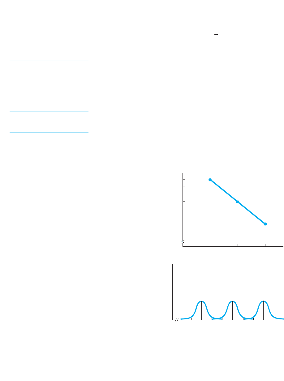
23. (a) The means for conditions 1, 2, and 3 are 15, 12, and

9, respectively.

(b)

©X 5 638, N 5 11, X

5 58

Noise level

Mean productivity

Low

Medium High

Productivity scores

μ for

high noise

μ for

medium

noise

μ for

low noise

(c)

(d) Apparently the relationship is that as noise level

increases, the typical productivity score decreases

from around 15 to around 12 to around 9.

25. (a) It is the variable that supposedly influences a

behavior; it is manipulated by the researcher.

(b) It reflects the behavior that is influenced by the inde-

pendent variable; it measures participants’ behavior.

27. (a) The independent variable.

(b) The dependent variable.

is an interval or ratio scale, a bar graph when the

independent variable is nominal or ordinal.

29. (a) Line graph; income on Y axis, age on X axis; find

median income per age group—income is skewed.

(b) Bar graph; positive votes on Y axis, presence or

absence of a wildlife refuge on X axis; find mean

number of votes, if normally distributed.

bohydrates consumed on X axis; find mean

running speed, if normally distributed.

(d) Bar graph; alcohol abuse on Y axis, ethnic group on

X axis; find mean rate of alcohol abuse per group, if

normally distributed.

Chapter 5

1. It is needed for a complete description of the data, indi-

cating how spread out scores are and how accurately the

mean summarizes them.

3. (a) The range is the distance between the highest and

lowest scores in a distribution.

(b) Because it includes only the most extreme and

often least-frequent scores, so it does not summa-

rize most of the differences in a distribution.

ratio scores that cannot be accurately described by

other measures.

5. (a) Variance is the average of the squared deviations

around the mean.

(b) Variance equals the squared standard deviation, and

the standard deviation equals the square root of the

variance.

7. Because a sample value too often tends to be smaller

than the population value. The unbiased estimates of the

population involve the quantity , resulting in a

slightly larger estimate.

9. (a) The lower score and the upper score ⫽

(b) The lower score and the upper score ⫽

and the upper score

11. (a) Range , so the scores spanned 8 dif-

ferent scores.

(b) , , , so

: The average squared deviation

of creativity scores from the mean of 4.10 is 6.29.

creativity scores from the mean of 4.10 is 2.51.

13. (a) With and , the scores are

, and 4.1 1 2.51 5 6.61.4.1 2 2.51 5 1.59

5 2.51X 5 4.1

5 16.29 5 2.51

168.12>10 5 6.29

5 1231 2N 5 10©X

5 231©X 5 41

5 8 2 0 5 8

5 ␮ 1 1s

.␮ 2 1s

5␮X

␮ 1 1σ

5 ␮ 2 1σ

X 1 1S

5 X 2 1S

N 2 1

(b) The portion of the normal curve between these

scores is 68%, so

15. (a) Because the sample tends to be normally distrib-

uted, the population should be normal too.

(b) Because , we would estimate

the to be 76.29.

(d) The estimated standard deviation is

(e) Between 72.19 and 80.39

17. (a) Guchi. Because his standard deviation is larger, his

scores are spread out around the mean, so he tends

to be a more inconsistent student.

(b) Pluto, because his scores are closer to the mean

of 60, so it more accurately describes all of his

scores.

mean score, and Pluto’s individual scores tend to be

closer to his mean than Guchi’s are to his mean.

(d) Guchi, because his scores vary more widely above

and below 60.

19. (a) Compute the mean and sample standard deviation

in each condition.

(b) Changing conditions A, B, C changes dependent

scores from around 11.00 to 32.75 to 48.00, respec-

tively.

and .71, respectively. These seem small, showing

little spread, so participants scored consistently in

each condition.

(d) Yes.

21. (a) Study A has a relatively narrow/skinny distribution,

and Study B has a wide/fat distribution.

(b) In A, about 68% of scores will be between

and ; in B, 68% will be

between and .

23. (a) For conditions 1, 2, and 3, we’d expect of about

13.33, 8.33, and 5.67, respectively.

(b) Somewhat inconsistently, because based

on we’d expect a of 4.51, 2.52, and 3.06,

respectively.

25. The shape of the distribution, a measure of central ten-

dency and a measure of variability.

27. (a) The flat line graph indicates that all conditions

produced close to the same mean, but a wide

variety of different scores was found throughout the

conditions.

(b) The mean for men was 14 and their standard

deviation was 3.

mate , and is estimating by using the sample

data to compute .s

␮

5 14

␮s

50140 1 10230140 2 102

45140 1 5235140 2 52

4.102

176.29 1176.29 2 4.102

116.85

5 4.10.

98,953.472>16 5 16.85.

199,223 2

␮

2 1297>17 5 76.29

1.1621100025 160.

1.682 1100025 680.

APPENDIX D / Answers to Odd-Numbered Questions 441

ANSWERS TO ODD-NUMBERED QUESTIONS

29. (a) A bar graph; rain/no rain on ; mean laughter time

on .

(b) A bar graph; divorced/not divorced on ; mean

weight change on .

income on .

(d) A line graph; amount paid on ; mean number of

ideas on .

(e) A line graph; number of siblings on ; mean vocab-

ulary size on .

(f) A bar graph; type of school on ; median income

rank on .

Chapter 6

1. (a) A z-score indicates the distance, measured in

standard deviation units, that a score is above

or below the mean.

(b) z-scores can be used to interpret scores from

any normal distribution of interval or ratio scores.

3. It is the distribution that results after transforming a

distribution of raw scores into z-scores.

5. (a) It is our model of the perfect normal z-distribution.

(b) It is used as a model of any normal distribution of

raw scores after being transformed to z-scores.

normally distributed, they should be from a contin-

uous interval or ratio variable, and the sample

should be relatively large.

7. (a) That it is normally distributed, that its equals the

of the raw score population, and that its standard

deviation (the standard error of the mean) equals

the raw score population’s standard deviation

divided by the square root of .

(b) Because it indicates the characteristics of any sam-

pling distribution, without our having to actually

measure all possible sample means.

9. (a) Convert the raw score to , use with the z-tables to

find the proportion of the area under the appropri-

ate part of the normal curve, and that proportion is

the rel. , or use it to determine percentile.

(b) In column B or C of the z-tables, find the specified

rel. or the rel. converted from the percentile, identify

the corresponding at the proportion, transform the

into its raw score, and that score is the cutoff score.

the sample mean into a z-score, follow the steps in

part (a) above.

11. (a) Small. This will give him a large positive z-score,

placing him at the top of his class.

(b) Large. Then he will have a small negative and be

relatively close to the mean.

13. , , and , so and

(a) For .

(b) For .X 5 6, z 5 16 2 8.582>1.98 521.30

X 5 10, z 5 110 2 8.582>1.98 51.72

5 8.58

5 1.98N 5 12©X

5 931©X 5 103

␮

442 APPENDIX D / Answers to Odd-Numbered Questions

15. (a) (b)

17. (a) (b)

(c)

(d)

19. From the z-table the 25th percentile is at approximately

. The cutoff score is then

21. To make the salaries comparable, compute . For

City A, For

City B, . City B

is the better offer, because her income will be closer to

(less below) the average cost in that city.

23. (a) , so of the curve is

between 60 and 56, plus of the curve below the

mean gives a total of or 69.15% of the curve

is expected to be below 60.

(b) , so of the curve is

between 54 and 56, plus of the curve that is

above the mean for a total of or 59.87%

scoring above 54.

above so the corresponding raw score is

25. (a) This is a rather infrequent mean.

(b) The sampling distribution of means.

27. (a) With normally distributed, interval, or ratio scores.

(b) With normally distributed, interval, or ratio scores.

29. (a)

(b) We are asking for its frequency.

(c)

(d)

Chapter 7

1. (a) In experiments the researcher manipulates one vari-

able and measures participants on another variable;

in correlational studies the researcher measures

participants on two variables.

(b) In experiments the researcher computes the mean of

the dependent ( ) scores for each condition of the

independent variable (each ); in correlational stud-

ies the researcher examines the relationship over all

pairs by computing a correlation coefficient.

3. You don’t necessarily know which variable occurred

first, nor have you controlled other variables that might

cause scores to change.

5. (a) A scatterplot is a graph of the individual data points

formed from a set of pairs.

(b) It is a data point that lies outside of the general

pattern in the scatterplot, because of an extreme

or score.

drawn through the center of the scatterplot.

X2Y

.70110025 70%

35>50 5 .70

.40 150025 200

X 5 11.8421821 56 5 62.72

z 51.84

1.20052.20

.5987

.50

.0987z 5 154 2 562>8 52.25

.6915

.50

.1915z 5 160 2 562>8 5 .50

z 5 170,000 2 85,0002>20,000 52.75

z 5 147,000 2 65,0002>15,000 521.2.

75 5 68.3

X 5 12.6721102 1z 52.67

.0250 1 .0250 5 .05

.3944 1 .4970 5 .8914

.0107.4706

z 522.0z 52.70

z 522.8z 511.0

7. (a) As the scores increase, the scores tend to

increase.

(b) As the scores increase, the scores tend to

decrease.

increase or only decrease.

9. (a) Particular scores are not consistently paired with

particular scores.

(b) The variability in at each is equal to the overall

variability in all scores in the data.

(d) Knowing does not improve accuracy in predict-

ing

11. (a) That the variable forms a relatively strong

relationship with ( is relatively large), so by

knowing someone’s we come close to knowing

his or her .

(b) That the variable forms a relatively weak rela-

tionship with ( is relatively small), so by know-

ing someone’s we have only a general idea if he

or she has a low or high score.

13. He is drawing the causal inference that more people

cause fewer bears, but it may be the number of hunters,

or the amount of pesticides used, or the noise level asso-

ciated with more people, etc.

15. (a) With , the scatterplot is skinnier.

(b) With , there is less variability in at

each .

more closely.

(d) No. He thought a positive was better than a nega-

tive . Consider the absolute value.

17. Disagree. Exceptionally smart people will produce a

restricted range of IQ scores and grade averages. With

an unrestricted range, the would be larger.

19. Compute r. , , ,

, , , , and

. .

This is a strong positive linear relationship, so a nurse’s

burnout score will allow reasonably accurate prediction

of her absenteeism.

21. Compute : ;

This is a very strong negative relationship, so that the

most dominant consistently weigh the most, and the less

dominant weigh less.

23. (a) Neither variable.

(b) Impossible to determine: being creative may cause

intelligence, or being intelligent may cause creativity,

or maybe something else (e.g., genes) causes both.

(d) We do not call either variable the independent

variable in a correlational coefficient.

25. (a) Correlational, Pearson .

(b) Experiment, with age as a (quasi-) independent

variable.

r 5 1 2 11872>990252.89.©D

5 312r

r 5 12853 2 25842>1146421344251.67N 5 9

©Y 5 3171©Y2

5 4624©Y

5 552©Y 5 68

1©X2

5 1444©X

5 212©X 5 38

Yr 52.40

r 52.40

(d) Correlational, Spearman after creating ranks for

number of visitors to correlate with attractiveness

rankings.

(e) Experiment.

Chapter 8

1. It is the line that summarizes a scatterplot by, on average,

passing through the center of the scores at each .

3. is the predicted score for a given , computed

from the regression equation.

5. (a) The intercept is the value of when the regres-

sion line crosses the axis.

(b) The slope indicates the direction and degree that the

regression line is slanted.

7. (a) The standard error of the estimate.

(b) It is a standard deviation, indicating the “average”

amount that the scores deviate from their corre-

sponding values of .

scores differ from the predicted scores, so it is

the “average” error.

9. is inversely related to the absolute value of .

Because a smaller indicates the scores are closer

to the regression line (and ) at each , which is what

happens with a stronger relationship (a larger ).

11. (a) is the coefficient of determination, or the propor-

tion of variance in that is accounted for by the

relationship with .

(b) indicates the proportional improvement in accu-

racy when using the relationship with to predict

scores, compared to using the overall mean of to

predict scores.

13. (a) Foofy; because is positive.

(b) Linear regression.

(d) , so our error is 19% smaller.

(e) The proportion of variance accounted for (the

coefficient of determination).

15. The researcher measured more than one variable and

then correlated them with one variable, and used the

to predict

17. (a) He should use multiple correlation and multiple

regression, simultaneously considering the hours

people study and their test speed when he predicts

error scores.

(b) With a multiple R of , : He will be

45% more accurate at predicting error scores when

considering hours studied and test speed than if

these predictors are not considered.

19. (a) Compute r:, ,

,, ,

and , so

.1.81

r 5 146002 40052>11565219492

5N 5 10

©XY 5 460,1©Y2

5 7921©Y

5 887©Y 5 89

1©X2

5 2025,©X

5 259©X 5 45

5 .451.67

Y.Xs

5 11.442

5 .19

5 3.90

XYY

APPENDIX D / Answers to Odd-Numbered Questions 443

ANSWERS TO ODD-NUMBERED QUESTIONS

(b) and

, so

attraction score of 9, the predicted anxiety score is

(d) Compute : , so

. The “average error” is 1.81

when using to predict anxiety scores.

21. (a) ;

, so

(b)

(c)

(d) ; very useful, providing a 45%

improvement in the accuracy of predictions

23. (a) The size of the correlation coefficient indirectly

indicates this, but the standard error of the estimate

most directly communicates how much better (or

worse) than predicted she’s likely to perform.

(b) Not very useful: Squaring a small correlation coef-

ficient produces a small proportion of variance

accounted for.

25. (a) Yes, by each condition.

(b) The and per condition.

27. (a) The independent ( ) variable.

(b) The dependent ( ) variable.

(d) The variance (or standard deviation) of that

condition.

29. (a) It is relatively strong.

(b) There is a high degree of consistency.

(d) The data points are close to the line,

(e) is relatively large.

(f) We can predict scores reasonably accurately.

Chapter 9

1. (a) It is our expectation or confidence in the event.

(b) The relative frequency of the event in the

population.

3. (a) Sampling with replacement is replacing the individ-

uals or events from a sample back into the popula-

tion before another sample is selected.

(b) Sampling without replacement is not replacing the

individuals or events from a sample before another

is selected.

replacement increases the probability of an event,

because there are fewer events that can occur; with

replacement, each probability remains constant.

5. It indicates that by chance, we’ve selected too

many high or low scores so that our sample is

5 1.672

5 .45

5 1.5824 1 5.11 5 7.43

5 2.06121 2 .67

5 1.53

5 .58X 1 5.112 1.58214.22225 5.11

a 5 7.556b 5 128532 25842>119082 144425.58

21 2 .81

5 1.81

5 13.0812S

5 3.081S

111.0529 1 4.18 5 13.63

5 111.052X 1 4.18.11.05214.525 4.18

a 5 8.9 2b 5 14600 2 40052>565 511.05

444 APPENDIX D / Answers to Odd-Numbered Questions

unrepresentative. Then the mean does not equal the

that it represents.

7. It indicates whether or not the sample’s z-score (and the

sample ) lies in the region of rejection.

9. The of a hurricane is . The uncle is

looking at an unrepresentative sample over the past

13 years. Poindexter uses the gambler’s fallacy, failing

to realize that p is based on the long run, and so in the

next few years there may not be a hurricane.

11. She had sampling error, obtaining an unrepresentative

sample that contained a majority of Poindexter sup-

porters, but the majority in the population were Dorcas

supporters.

13. (a) .

(b) Yes: , so

population.

(d) Because such a sample and mean is unlikely to

occur if we are representing this population.

15. (a)

(b) Yes: , so .

population.

(d) Reject that the sample represents this population.

17. , so . No,

this z-score is beyond the critical value of , so this

sample is unlikely to be representing this population.

19. No, the gender of one baby is independent of another,

and a boy now is no more likely than at any other time,

with .

21. (a) For Fred’s sample, , and for Ethel’s, .

(b) The population with is most likely to pro-

duce a sample with , and the population

with is most likely to produce a sample

with .

23. (a) The ; .

Then . With a

critical value of , conclude that the football

players do not represent this population.

(b) Football players, as represented by your sample,

form a population different from non-football play-

ers, having a of about 35.67.

25. (a)

(b)

(c)

(d)

(e) For each the probability equals the above rel. f.

27. (a)

(b) p 5 .0793

21.41; rel. f 5 .0793

z 5 146 2 502>2.8 5σ

5 18>140 5 2.846;

rel. f 5 .1056 1 .2266 5 .33221.75,

z 5 149 2 432>8 5z 5 133 2 432>8 521.25,

rel. f 5 .0517 1 .0517 5 .10341.13,

z 5 144 2 432>8 5z 5 142 2 432>8 52.13,

z 5 151 2 432>8 511.0, rel. f 5 .1587

z 5 127 2 432>8 522.0, rel. f 5 .0228

␮

;1.96

z 5 135.67 2 302>1.67 513.40

5 5>19, 5 1.67X 5 321>9 5 35.67

5 18

␮ 5 18

5 26

␮ 5 26

␮ 5 18␮ 5 26

p 5 .5

;1.96

z 5 134 2 282>1.521 513.945σ

5 1.521

z 5 136.8 2 332>2.19 5 1.74σ

5 2.19

11.645

z 5 172.1 2 752>1.28 522.27,σ

5 1.28

11.96

160>2005 5 .80p

␮

Chapter 10

1. A sample may (1) poorly represent one population

because of sampling error, or (2) represent some other

population.

3. stands for the criterion probability; it determines the

size of the region of rejection and the theoretical proba-

bility of a Type I error.

5. They describe the predicted relationship that may or

may not be demonstrated in an experiment.

7. (a) Use a one-tailed test when predicting the direction

the scores will change.

(b) Use a two-tailed test when predicting a relationship

but not the direction that scores will change.

9. (a) Power is the probability of not making a Type II

error.

(b) So we can detect relationships when they exist and

thus learn something about nature.

missed a real relationship.

(d) In a one-tailed test the critical value is smaller than

in a two-tailed test; so the obtained value is more

likely to be significant.

11. (a) We will demonstrate that changing the independent

variable from a week other than finals week to

finals week increases the dependent variable of

amount of pizza consumed; we will not demon-

strate an increase.

(b) We will demonstrate that changing the independ-

ent variable from not performing breathing exer-

cises to performing them changes the dependent

variable of blood pressure; we will not demon-

strate a change.

variable by increasing hormone levels changes the

dependent variable of pain sensitivity; we will not

demonstrate a change.

(d) We will demonstrate that changing the independent

variable by increasing amount of light will decrease

the dependent variable of frequency of dreams; we

will not demonstrate a decrease.

13. (a) A two-tailed test because we do not predict the

direction that scores will change.

(b) ,

(c)

(d)

(e) Yes, because is beyond , the results are sig-

nificant: Changing from the condition of no music

to the condition of music results in test scores

changing from a of 50 to a of around 54.63.

15. (a) The probability of a Type I error is . The

error would be concluding that music influences

scores when really it does not.

p 6 .05

␮␮

crit

obt

crit

5 ;1.96

obt

5 154.63 2 502>1.71 512.71

5 12>249 5 1.71;

: ␮ ? 50H

: ␮ 5 50

␣

(b) By rejecting , there is no chance of making a

Type II error. It would be concluding that music

does not influence scores when really it does.

17. She is incorrect about Type I errors, because the total

size of the region of rejection (which is ) is the same

regardless of whether a one- or two-tailed test is used;

is also the probability of making a Type I error, so it

is equally likely using either type of test.

19. (a) She is correct; that is what indicates.

(b) She is incorrect. In both studies the researchers

decided the results were unlikely to reflect sam-

pling error from the population; they merely

defined unlikely differently.

21. (a) The researcher decided that the difference between

the scores for brand X and other brands is too large

to have resulted by chance if there wasn’t a real

difference between them.

(b) The indicates an of , so the proba-

bility is that the researcher made a Type I

error. This p is far too large for us to accept the

conclusion.

23. (a) One-tailed.

(b) : The of all art majors is less than or equal

to that of engineers who are at 45; : the of

all art majors is greater than that of engineers

who are at 45.

(c)

This is not larger than ; the results are

not significant.

(d) We have no evidence regarding whether, nation-

wide, the visual memory ability of the two groups

differs or not.

(e) .

25. (a) The independent variable is manipulated by the

researcher; the dependent variable measures parti-

cipants’ scores.

(b) Dependent variable.

but an interval variable allows negative scores;

nominal variables are categorical variables; ordinal

scores are the equivalent of 1st, 2nd, etc.

(d) A normal distribution is bell shaped and symmetri-

cal with two tails; a skewed distribution is asym-

metrical with only one pronounced tail.

27. This will produce two normal distributions on the same

axis, with the morning’s centered around a of 40 and

the evening’s centered around a of 60.

29. (a) Because they study the laws of nature and a rela-

tionship is the telltale sign of a law at work.

(b) A real relationship occurs in nature (in the “popula-

tion”). One produced by sampling error occurs by

chance, and only in the sample data.

␮

z 511.43, p 7 .05

crit

511.645

obt

5 149 2 452>2.8 511.428.σ

514>125 5 2.8;

␮H

.44

.44␣p 6 .44

p 6 .0001

␣

APPENDIX D / Answers to Odd-Numbered Questions 445

ANSWERS TO ODD-NUMBERED QUESTIONS

Chapter 11

1. (a) The t-test and the z-test.

(b) Compute z if the standard deviation of the raw

score population ( ) is known; compute t if is

estimated by .

ratio dependent scores, and the scores are approxi-

mately normally distributed.

3. (a) is the estimated standard error of the mean; is

the true standard error of the mean.

(b) Both are used as a “standard deviation” to locate

a sample mean on the sampling distribution of

means.

5. (a)

(b)

ing it to the appropriate critical value; if the coeffi-

cient is significant, compute the regression equation

and graph it, compute the proportion of variance

accounted for, and interpret the relationship.

7. To describe the relationship and interpret it psychologi-

cally, sociologically, etc.

9. (a) Power is the probability of rejecting when it is

false (not making a Type II error).

(b) When a result is not significant.

(d) When designing a study.

11. (a) ;

(b)

(d) Using this book rather than other books produces

a significant improvement in exam scores:

(e)

13. (a)

(b)

(d) , so the results are not signif-

icant, so do not compute the confidence interval.

(e) She has no evidence that the arguments change peo-

ple’s attitudes toward this issue.

15. Disagree. Everything Poindexter said was meaningless,

because he failed to first perform significance testing to

eliminate the possibility that his correlation was merely

a fluke resulting from sampling error.

17. (a) ;

(b) With .

(c)

(d) The correlation is significant, so he should con-

clude that the relationship exists in the population,

and he should estimate that is approximately

(e) The regression equation and should be computed.r

1.38

␳

r170251.38, p 6 .05 1and even, 6 .012

df 5 70, r

crit

5 ;.232

: ␳ ? 0H

: ␳ 5 0

t17251.39, p 7 .05

df 5 7, t

crit

5 ;2.365

obt

5 153.25 2 502>8.44 51.39

: ␮ ? 50H

: ␮ 5 50

78.5 5 70.33 # ␮ # 86.67

112.2622 113.612122.26221 78.5 # ␮ # 13.612

2.77, p 6 .05

obt

1925

df 5 9, t

crit

5 ;2.262

obt

5 178.5 2 68.52>3.61 512.77

5 130.5; s

5 1130.5>10 5 3.61;

: ␮ ? 68.5H

: ␮ 5 68.5

␳

446 APPENDIX D / Answers to Odd-Numbered Questions

19. ; ; , ;

;

. The results are significant, so

there is evidence of a relationship: Without uniforms,

; with uniforms, is around 8.67. The 95% con-

fidence interval is

so with uniforms is between

6.40 and 10.94.

21. (a)

(b)

23. The df of 80 is .33 of the distance between the df at 60 and

120, so the target is .33 of the distance from 2.000 to

1.980: , so ,

and thus equals the target of 1.993.

25. (a) We must first believe that it is a real relationship,

which is what significant indicates.

(b) Significant means only that we believe that the rela-

tionship exists in the population; a significant rela-

tionship is unimportant if it accounts for little of the

variance.

27. The z- and t-tests are used to compare the of a popula-

tion when exposed to one condition of the independent

variable, to the scores in a sample that is exposed to a dif-

ferent condition. A correlation coefficient is used when

we have measured the and scores of a sample.

29. (a) They are equally significant.

(b) Study B’s is larger.

pling distribution.

(d) The probability of a Type I error is .031 in A, but

less than .001 in B.

31. (a) Compute the mean and standard deviation for each set

of scores, compute the Pearson between the scores

and test if it is significant (two-tailed). If so, perform

linear regression. The size of (and ) is the key.

(b) We have the mean and (estimated) standard devia-

tion, so perform the two-tailed, one-sample t-test,

comparing the to Whether

is significant is the key. Then compute the confi-

dence interval for the represented by the sample.

tion for this year’s team. Perform the one-tailed

z-test, comparing to . Whether

is significant is the key.

Chapter 12

1. (a) The independent-samples t-test and the related-

samples t-test.

(b) Whether the scientist created independent samples

or related samples.

3. (a) Each score in one sample is paired with a score in

the other sample by matching pairs of participants

or by repeatedly measuring the same participants in

all conditions.

obt

␮ 5 71.1X 5 77.6

␮

obt

␮ 5 106.X 5 97.4

␮

crit

2.000 2 .0066

1.02021.3325 .00662.000 2 1.980 5 .020

crit

t152521.72, p 7 .05

t1422516.72, p 6 .05

␮1.882212.57121 8.67,

1.8822122.57121 8.67 # ␮ #

␮␮ 5 12

df 5 5, t

crit

5 ;2.571

obt

5 18.667 2 122>.882 523.78;14.67>6 5 .882

5 4.67X 5 8.667H

: ␮ ? 12H

: ␮ 5 12

(b) The scores are interval or ratio scores; the popula-

tions are normal and have homogeneous variance.

5. (a) is the standard error of the difference—the

“standard deviation” of the sampling distribution

of differences between means from independent

samples.

(b) is the standard error of the mean difference, the

“standard deviation” of the sampling distribution of

from related samples.

number of scores in the experiment.

7. It indicates a range of values of , one of which is

likely to represent.

9. (a) It indicates the size of the influence that the inde-

pendent variable had on dependent scores.

(b) It measures effect size using the magnitude of the

difference between the means of the conditions.

dependent scores accounted for by changing the

conditions of the independent variable in the exper-

iment, indicating how consistently close to the

mean of each condition the scores are.

11. She should graph the results, compute the appropriate

confidence interval, and compute the effect size.

13. (a) : ; :

(b) ; ;

obt

5 143 2 392>1.78 512.25

5 1.78s

pool

5 23.695

␮

2 ␮

? 0H

␮

2 ␮

5 0H

D␮

(d) The results are significant. In the population, chil-

dren exhibit more aggressive acts after watching the

show (with about 3.9), than they do before the

show (with about 2.7).

(e)

(f) ; a relatively large difference.

19. You cannot test the same people first when they’re

males and then again when they’re females.

21. (a) Two-tailed.

(b) , H

␮

2 ␮

? 0H

: ␮

2 ␮

5 0

d 5 1.2>11.289

5 1.14

1.2 5 .39 # ␮

# 2.01112.26221

1.3592122.26221 1.2 # ␮

# 1.3592

␮

APPENDIX D / Answers to Odd-Numbered Questions 447

ANSWERS TO ODD-NUMBERED QUESTIONS

(d) The results are significant: In the population, hot

baths (with about 43) produce different relax-

ation scores than cold baths (with about 39).

(e)

(f)

This is a

moderate to large effect.

(g) Label the axis as bath temperature; label the

axis as mean relaxation score; plot the data point

for cold baths at a of 39 and for hot baths at a of

43; connect the data points with a straight line.

15. (a) : ; :

(b)

much sunshine exhibit a significantly higher well-

being score than when exposed to less sunshine.

(d)

(e) The of 15.5, the of 18.13.

(f) ; they are on

average about 64% more accurate.

(g) By accounting for 64% of the variance, these

results are very important.

17. (a) : ;

(b) , ,

crit

511.833df 5 9

obt

5 11.2 2 02>.359 513.34

5 .359;s

5 1.289D 5 1.2

: ␮

7 0␮

# 0H

5 13.512

>313.512

1 745 .64

.86 # ␮

# 4.40

crit

5 ;2.365df 5 7

obt

5 12.63 2 02>.75 513.51

␮

? 0H

␮

5 0H

5 12.252

>312.252

1 2845 .15.

d 5 143 2 392>123.695

5 .82;

112.04821 4 5 .35 # ␮

2 ␮

# 7.65

11.782122.048021 4 # ␮

2 ␮

# 11.782

␮

crit

5 ; 2.048.df 5 115 2 121 115 2 125 28

(c),; ,,

With , , so is

significant.

(d)

(e) Police who’ve taken this course are more success-

ful at solving disputes than police who have not

taken it. The for the police with the course is

around 14.1, and the for police without the

course is around 11.5. The absolute difference

between these s will be between 4.76 and .44.

(f) ; ; taking the course is important.

23. The independent variable is manipulated by the

researcher to create the conditions in which participants

are tested; presumably this will cause a behavior to

change. The dependent variable measures the behavior

of participants that is to be changed.

25. (a) When the dependent variable is measured using

normally distributed, interval, or ratio scores, and

has homogeneity of variance.

(b) z-test, performed in a one-sample experiment

when and under one condition are known;

one sample t-test, performed in a one-sample

experiment when under one condition is known

but must be estimated using ; independent

samples t-test, performed when independent sam-

ples of participants are tested under two condi-

tions; related samples t-test, performed when

participants are tested under two conditions of the

independent variable, with either matching pairs

of participants or with repeated measures of the

same participants.

27. (a) To predict scores by knowing someone’s score.

(b) We predict the mean of a condition for participants

in that condition.

(d) When the predicted mean score is close to most par-

ticipants’ actual score.

29. A confidence interval always uses the two-tailed .t

crit

␮

5 .26d 5 1.13

␮

112.1012122.6 524.76 # ␮

2 ␮

#2.44

11.032122.1012122.6 # ␮

2 ␮

# 11.032

obt

crit

5 ;2.101df 5 18522.52

obt

5 111.5 214.12>1.03s

5 1.03s

pool

5 5.29

5 5.86X

5 14.1s

5 4.72X

5 11.5