Heiman G. Basic Statistics for the Behavioral Sciences

Подождите немного. Документ загружается.

268 CHAPTER 12 / The Two-Sample t-Test

– X

–3.0 –2.0 –1.0

0 +1.0 +2.0 +3.0

– X

–t

crit

= –2.042 +t

crit

= +2.042 +t

obt

= +2.93

Differences:

Values of t:

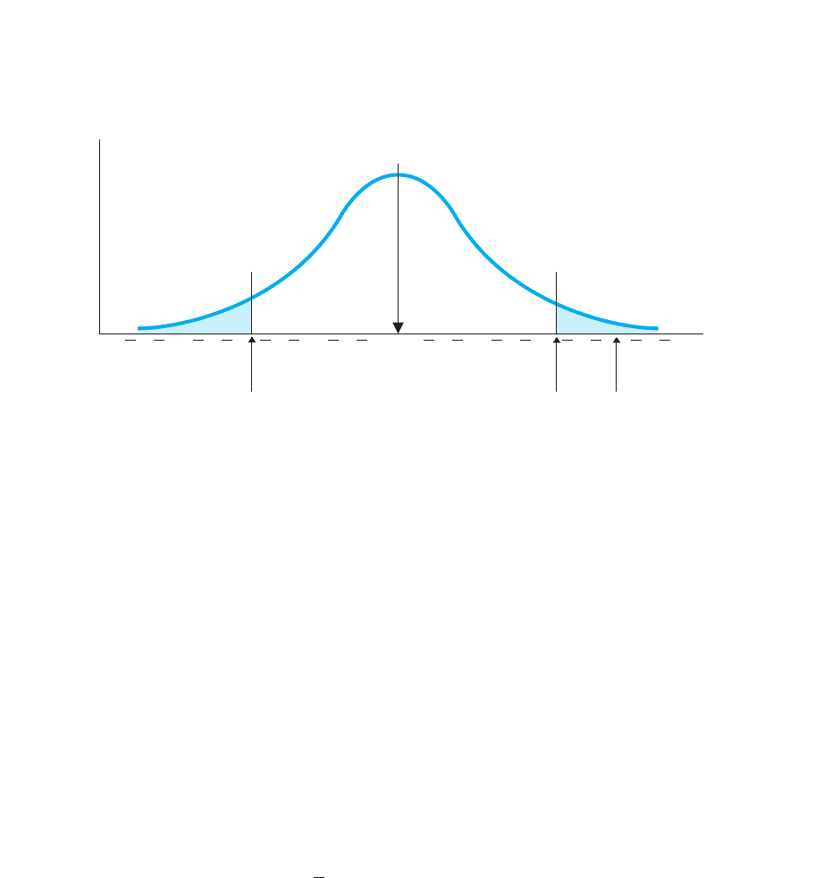
FIGURE 12.3

sampling distribution of differences between means when . A larger t indicates a larger

difference between means.

The shows the location of a difference of 3.01t

obt



2 

5 0

of 2.93 lies beyond , so the results are significant: Our difference of is so

unlikely to occur if our samples were representing no difference in the population that

we reject that this is what they represent. Therefore, we reject and accept the that

we are representing a difference between that is not zero.

We can say that our difference of is significantly different from 0. Or we can say

that our two means differ significantly from each other. Here, the mean for hypnosis

(23) is larger than the mean for no hypnosis (20), so we can conclude that increasing

the amount of hypnosis leads to significantly higher recall scores.

If was not beyond , we would not reject , and we would have no evidence

for or against a relationship between hypnosis and recall. Then we would consider if

we had sufficient power to prevent a Type II error (retaining a false ). As in the pre-

vious chapter, we maximize power here by designing the study to (1) maximize the size

of the difference between the means, (2) minimize the variability of scores within each

condition, and (3) maximize the size of . These steps will maximize the size of

relative to so that we are unlikely to miss the relationship if it really exists.

Because we did find a significant result, we describe and interpret the relationship.

First, from our sample means, we expect the for no hypnosis to be around 20 and the

for hypnosis to be around 23. To more precisely describe these , we could com-

pute a confidence interval for each. To do so, we would use the formula for a confi-

dence interval in the previous chapter, looking at only one condition at a time, using

only one and , and computing a new standard error and Then we’d know the

range of values of likely to be represented by each of our means.

However, another way to describe the populations represented by our samples is to

create a confidence interval for the difference between the .

Confidence Interval for the Difference between Two s

Above we found a difference of between our sample means, so if we could exam-

ine the corresponding and , we’d expect their difference would be around

To more precisely define “around,” we can compute a confidence interval for this

difference. We will compute the largest and smallest difference between that our

difference between sample means is likely to represent. Then we will have a range of

s

13.



␮

s



crit

.Xs

s



crit

obt

crit

obt

s

13t

crit

differences between the population that our difference between may represent.

The confidence interval for the difference between two ␮s describes a range of dif-

ferences between two , one of which is likely to be represented by the difference

between our two sample means.

␮s

s␮s

Here, stands for the unknown difference we are estimating. The is the two-

tailed value found for the appropriate at . The values of

and are computed in the t-test.

In the hypnosis study, the two-tailed for and is ,

, and . Filling in the formula gives

Multiplying 1.023 times gives

So, finally,

Because , this is the 95% confidence interval: We are 95% confident that the

interval between and 5.089 contains the difference we’d find between the for

no hypnosis and hypnosis. In essence, if someone asked us how big a difference hyp-

nosis makes for everyone in the population when recalling information in our study,

we’d be 95% confident that the difference is, on average, between about and 5.09

correct answers.

Performing One-Tailed Tests with Independent Samples

As usual, we perform a one-tailed test whenever we predict the specific direction in

which the dependent scores will change. Thus, we would have performed a one-tailed

test if we had predicted that hypnosis would increase recall scores. Everything dis-

cussed previously applies here, but to prevent confusion, we’ll use the subscript h for

hypnosis and n for no hypnosis. Then follow these steps:

1. Decide which and corresponding is expected to be larger. (We predict the

for hypnosis is larger.)

2. Arbitrarily decide which condition to subtract from the other. (We’ll subtract no

hypnosis from hypnosis.)

3. Decide whether the predicted difference will be positive or negative. (Subtracting

the smaller from the larger should produce a positive difference, greater

than zero.)

4. Create and to match this prediction. (Our is that ; is

that .)␮

2 ␮

# 0

␮

2 ␮

7 0H

␮

␮X

.91

␮s.911

␣ 5 .05

.911 # ␮

2 ␮

# 5.089

22.089 1 1132# ␮

2 ␮

#12.089 1 1132

;2.042

11.0232122.04221 1132# ␮

2 ␮

# 11.0232112.04221 1132

2 X

513s

5 1.023

;2.042␣ 5 .05df 5 30t

crit

2 X

df 5 1n

2 121 1n

2 12␣

crit

␮

2 ␮

The formula for the confidence interval for the difference

between two ␮s is

212t

crit

21 1X

2 X

2# ␮

2 ␮

# 1s

211t

crit

21 1X

2 X

The Independent-Samples t-Test 269

270 CHAPTER 12 / The Two-Sample t-Test

5. Envision the same sampling distribution that we used in the two-tailed test. Obtain

the one-tailed from Table 2 in Appendix C. Locate the region of rejection

based on your prediction. If we expect a positive difference, it is in the right-hand

tail of the sampling distribution, so is positive. If we predict a negative differ-

ence, it is in the left-hand tail and is negative.

6. Compute as we did previously, but be sure to subtract the in the same way

as in . (We used , so we’d compute .)

Conversely, if we had predicted that hypnosis would decrease scores, subtracting

, we would have and , and would be

negative.

SUMMARY OF THE INDEPENDENT-SAMPLES t-TEST

After checking that the study meets the assumptions, the independent-samples t-test

involves the following:

1. Create either the two-tailed or one-tailed H

and H

2. Compute :

a. Compute , , and ; , , and .

b. Compute the pooled variance .

c. Compute the standard error of the difference .

d. Compute .

3. Find : In the t-tables, use .

4. Compare to : If is beyond , the results are significant; describe the

relationship. If is not beyond , the results are not significant; make no

conclusion about the relationship.

5. Compute the confidence interval: Describe the represented by each condition

and/or the difference between the .s



crit

obt

crit

obt

crit

obt

df 5 1n

2 121 1n

2 12t

crit

obt

pool

obt

crit

: 

2 

$ 0H

: 

2 

6 0h 2 n

2 X



2 

Xst

obt

crit

■

Perform the independent-samples t-test in

experiments that test two independent samples.

MORE EXAMPLES

We perform a two-tailed experiment, so :

and . The ,

, , , , and .

Then

11329 1 11529.4

13 1 15

5 9.214

pool

2 12s

1 1n

2 12s

2 121 1n

2 12

5 16s

5 9.4X

5 21n

5 14s

5 9

5 24H

:

2 

? 0

2 

5 0

With and ,

The is significant: We expect 

obt

crit

5 ;2.048.

df 5 1n

2 121 1n

2 125 28 5 .05

512.70

obt

2 X

22 1

2 

124 2 2122 0

1.111

9.214 a

b5 1.111

pool

A QUICK REVIEW

(continued)

THE RELATED-SAMPLES t-TEST

Now we will discuss the other version of the two-sample t-test. The related-samples

t-test is the parametric procedure used with two related samples. Related samples

occur when we pair each score in one sample with a particular score in the other sam-

ple. Researchers create related samples to have more equivalent and thus more compa-

rable samples. Two types of research designs produce related samples. They are

matched-samples designs and repeated-measures designs.

In a matched-samples design, we match each participant in one condition with a

participant in the other condition. For example, say that we want to measure how well

people shoot baskets when using either a standard basketball or a new type of ball (one

with handles). If, however, by luck, one condition contained taller people than the

other, then differences in basket shooting could be due to the differences in height

instead of the different balls. The solution is to create two samples containing people

who are the same height. We do this by matching pairs of people who are the same

height and assigning a member of the pair to each condition. Thus, if two participants

are 6 feet tall, one will be assigned to each condition. Likewise, a 4-foot person in one

condition is matched with a 4-footer in the other condition, and so on. This will pro-

duce two samples that, overall, are equivalent in height, so any differences in basket

shooting between them cannot be due to differences in height. Likewise, we might

match participants using age, or physical ability, or we might use naturally occurring

pairs such as roommates or identical twins.

The other, more common, way of producing related samples is called repeated meas-

ures. In a repeated-measures design, each participant is tested under all conditions of

the independent variable. For example, we might first test people when they use the

standard basketball and then measure the same people again when they use the new

ball. (Although we have one sample of participants, we have two samples of scores.)

Here, any differences in basket shooting between the samples cannot be due to differ-

ences in height or to any other attribute of the participants.

to be around 24 and to be around 21. The confi-

dence interval for the difference between the is

(1.111)(2.048)  3  





(1.111)(2.048)  3

For Practice

We test whether “cramming” for an exam is harmful

to grades. Condition 1 crams for a pretend exam,

but condition 2 does not. Each , the cramming

is 43 , and the no-cramming is 48

.1s

5 83.62

X1s

5 642X

n 5 31

0.725 # 

2 

# 5.275

211t

crit

21 1X

2 X

212t

crit

21 1X

2 X

2# 

2 

s



1. Subtracting cramming from no cramming, what

are and ?

2. Will be positive or negative?

3. Compute .

4. What do you conclude about this relationship?

5. Compute the confidence interval between .

Answers

1. ;

2. Positive

3. ;

;

4. With and , , is signifi-

cant: is around 43; is around 48.

5. (2.19)(2.00)  5 





 (2.19)(2.000)  5

 0.62 





 9.38



obt

crit

511.671df 5 60 5 .05

obt

5 152>2.190 512.28

5 173.801.06525 2.190

pool

5 11920 1 25082>60 5 73.80

: 

2 

# 0H

: 

2 

7 0

s

obt

crit

The Related-Samples t-Test 271

272 CHAPTER 12 / The Two-Sample t-Test

Matched-groups and repeated-measures designs are analyzed in the same way be-

cause both produce related samples. Related samples are also called dependent sam-

ples. In Chapter 9, two events were dependent when the probability of one is influenced

by the occurrence of the other. Related samples are dependent because the probability

that a score in a pair is a particular value is influenced by the paired score. For exam-

ple, if I make zero baskets in one condition, I’ll probably make close to zero in the

other condition. This is not the case with independent samples: In the hypnosis study,

whether someone scores 0 in the no-hypnosis condition will not influence the probabil-

ity of anyone scoring 0 in the hypnosis condition.

We cannot use the independent-samples t-test in such situations because its sampling

distribution describes the probability of differences between means from independent

samples. With related samples, we must compute this probability differently, so we cre-

ate the sampling distribution differently and we compute differently. However,

except for requiring related samples, the assumptions of the related-samples t-test are

the same as those for the independent-samples t-test: (1) The dependent variable

involves an interval or ratio scale, (2) the raw score populations are at least approxi-

mately normally distributed, and (3) the populations have homogeneous variance.

Because related samples form pairs of scores, the in the two samples must be equal.

The Logic of Hypotheses Testing in the

Related-Samples t-Test

Let’s say that we are interested in phobias (irrational fears of objects or events). We

have a new therapy we want to test on spider-phobics—people who are overly fright-

ened by spiders. From the local phobia club, we randomly select the unpowerful of

five spider-phobics and test our therapy using repeated measures of two conditions:

before therapy and after therapy. Before therapy we measure each person’s fear

response to a picture of a spider by measuring heart rate, perspiration, and so on. Then

we compute a “fear” score between 0 (no fear) and 20 (holy terror!). After providing

the therapy, we again measure the person’s fear response to the picture. (A before-and-

after, or pretest/posttest, design such as this always uses the related-samples t-test.)

Say that we obtained the raw scores shown on the left side of Table 12.3. First, com-

pute the mean of each condition (each column). Before therapy the mean fear score is

14.80, but after therapy the mean is 11.20. Apparently, the therapy reduced fear scores

by an average of points. But, on the other hand, maybe therapy

does nothing; maybe this difference is solely the result of sampling error from the one

population of fear scores we’d have with or without therapy.

14.80 2 11.20 5 3.6

obt

Before After

Participant Therapy ⴚ Therapy ⴝ DD

1 (Foofy) 11  8 39

2 (Biff) 16  11 525

3 (Cleo) 20  15 525

4 (Attila) 17  11 636

5 (Slug) 10  11 11

㛬㛬㛬㛬㛬㛬㛬㛬㛬㛬㛬㛬㛬

14.80 11.20 D  18 D

 96

N  5 3.6D

©©X

5X 5

TABLE 12.3

Finding the Difference

Scores in the Phobia

Study

Each D  Before  After

To test these hypotheses, we first transform the data and then perform a t-test on

the transformed scores. As shown in Table 12.3, we transform the data by first find-

ing the difference between the two raw scores for each participant. This difference

score is symbolized by Here, we subtracted after therapy from before therapy. You

could subtract in the reverse order, but subtract all scores in the same way. If this

were a matched-samples design, we’d subtract the scores from each pair of matched

participants.

Next, compute the mean difference, symbolized as . Add the positive and negative

differences to find the sum of the differences, symbolized by . Then divide by , the

number of difference scores. In Table 12.3, equals , which is . Notice that

this is also the difference between our original means of 14.80 and 11.20. Anyway you

approach it, the before scores were, on average, 3.6 points higher than the after scores.

(As in the far right-hand column of Table 12.3, later we’ll need to square each differ-

ence and then find the sum, finding .)

Now here’s the strange part: Forget about the before and after scores for the

moment and consider only the difference scores. We have one sample mean from

one random sample of scores. As in the previous chapter, with one sample we perform

the one-sample t-test! The fact that we have difference scores is irrelevant, so we cre-

ate the statistical hypotheses and test them in virtually the same way that we did with

the one-sample t-test.

REMEMBER The related-samples t-test is performed by applying the one-

sample t-test to the difference scores.

STATISTICAL HYPOTHESES FOR THE RELATED-SAMPLES t-TEST

Our sample of difference scores represents the population of difference scores that

would result if we could measure the population’s fear scores under each condition and

then subtract the scores in one population from the corresponding scores in the other

population. The population of difference scores has a that we identify as To cre-

ate the statistical hypotheses, we determine the predicted values of in and .

In reality, we expect the therapy to reduce fear scores, but let’s first perform a two-

tailed test. always says no relationship is present, so it says the population of before-

scores is the same as the population of after-scores. However, when we subtract them

as we did in the sample, not every will equal zero because, due to random physiolog-

ical or psychological fluctuations, some participants will not score identically when

tested before and after. Therefore, we will have a population of different , as shown

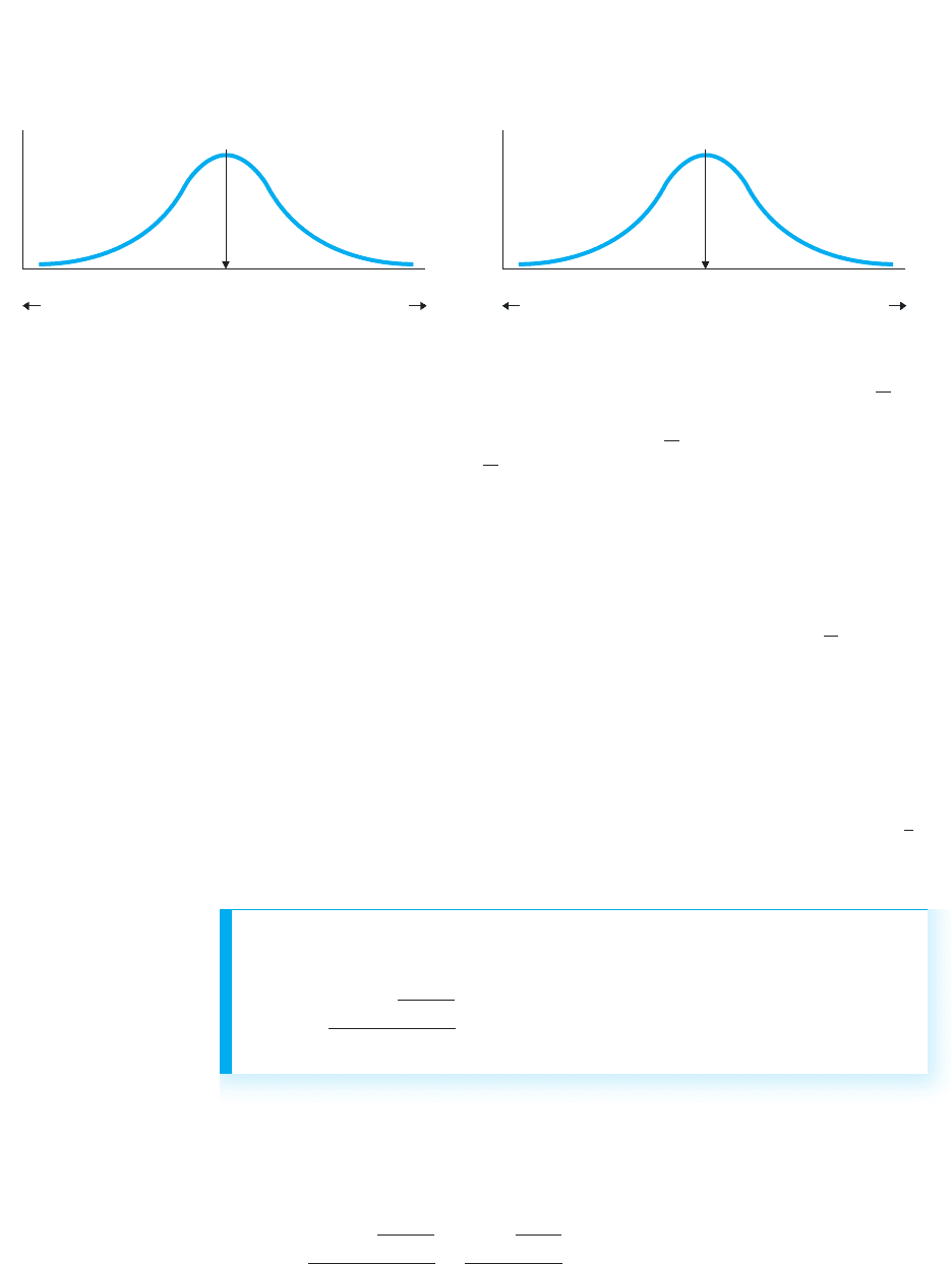
on the left in Figure 12.4.

On average, the positive and negative differences should cancel out to produce a

. This is the population that says that our sample of represents, and that

our somewhat poorly represents this . Therefore, .

For the alternative hypothesis, if the therapy alters fear scores in the population, then

either the before scores or the after scores will be consistently higher. Then, after sub-

tracting them, the population of will tend to contain only positive or only negative

scores. Therefore, the average difference will be a positive or negative number,

and not zero. Thus, .

We test by examining the sampling distribution, which here is the sampling

distribution of mean differences. Shown on the right side of Figure 12.4, it is as if we

infinitely sampled the population of on the left that says our sample represents.H

: 

? 0

1

: 

5 0

DsH



5 0



.

©D

13.618>5D

N©D

Statistical Hypotheses for the Related-Samples t-Test 273

274 CHAPTER 12 / The Two-Sample t-Test

Larger positive Ds

Larger negative Ds

Distribution of difference scores

DDD

DDDD

0 D

DDDD

Larger positive D

–

Larger negative D

–

Distribution of mean differences

–

0 D

–

FIGURE 12.4

Population of difference scores described by H

and the resulting sampling distribution of mean differences

The sampling distribution of mean differences shows all possible values of that

occur when samples are drawn from a population of difference scores where .

For the phobia study, it essentially shows all values of we might get by chance when

the therapy does not work. The that are farther into the tails of the distribution are

less likely to occur if was true and the therapy did not work.

Notice that the hypotheses and and the above sampling dis-

tribution are appropriate for the two-tailed test for any study when testing whether the

data represent zero difference between your conditions. This is the most common

approach and the one that we’ll discuss. (Consult an advanced statistics book to test for

nonzero differences.)

We test our by determining where on the sampling distribution our is located.

To do so, we compute .

Computing the Related-Samples t-Test

Computing here is identical to computing the one-sample t-test discussed in

Chapter 11—only the symbols have been changed from to There, we first com-

puted the estimated population variance , then the standard error of the mean ,

and then . We perform the same three steps here.

First, find , which is the estimated population variance of the difference scores.s

obt

21s

obt

: 

? 0H

: 

5 0



5 0

(Note: For all computations in this t-test, equals the number of difference scores.)

Using the data from the phobia study in Table 12.3, we have

©D

1©D2

N 2 1

96 2

1182

5 7.80

The formula for is

©D

1©D2

N 2 1

Second, find . This is the standard error of the mean difference, or the “stan-

dard deviation” of the sampling distribution of . (Just as was the standard deviation

of the sampling distribution when we called the mean .)X

Divide by and then find the square root. For the phobia study, and

, so

Third, find .t

obt

7.80

5 21.56 5 1.249

N 5 5

5 7.80Ns

Here, is the mean of your difference scores, is computed as above, and is the

value given in : It is always zero (unless you are testing a nonzero difference). Then,

as usual, is like a z-score, indicating how far our is from the of the sampling

distribution when measured in standard error units.

For the phobia study, , and . Filling in the formula, we

have

Thus, .

Interpreting the Related-Samples t-Test

Interpret by comparing it to from the t-tables in Appendix C. Here, .

REMEMBER The degrees of freedom in the related-samples t-test are

, where is the number of difference scores.

For the phobia study, with and , the two-tailed is .

The completed sampling distribution is shown in Figure 12.5. The is in the region

of rejection, so the results are significant: Our sample with is so unlikely

to be representing the population of where that we reject the that ourH

␮

5 0Ds

D 513.6

obt

;2.776t

crit

df 5 5–1 5 4␣ 5 .05

Ndf 5 N 2 1

df 5 N 2 1t

crit

obt

512.88

obt

2 ␮

13.6 2 0

1.249

512.88

␮

5 0s

5 1.249D 5 3.6

␮

obt

␮s

The formula for the standard error of the mean difference is

The formula for the related-samples t-test is

obt

2 ␮

Statistical Hypotheses for the Related-Samples t-Test 275

276 CHAPTER 12 / The Two-Sample t-Test

DDDDDDD0 DD DDDDD

obt

= +2.88

(D = +3.6)

crit

= +2.776+t

crit

= –2.776

Values of t

Larger positive Ds

...

–2.0 –1.0

0 +1.0 +2.0 ...

Larger negative Ds

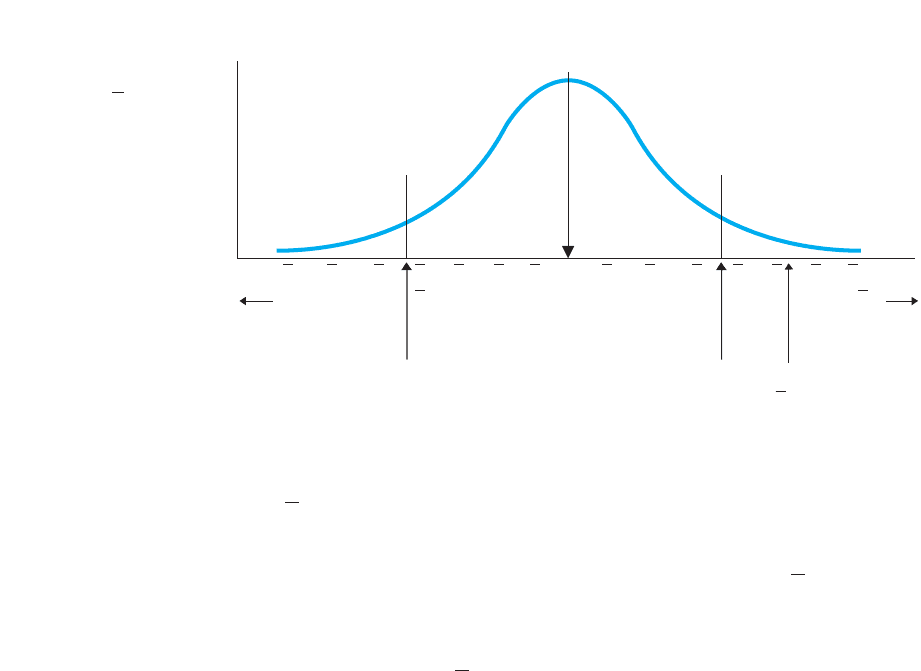
FIGURE 12.5

Two-tailed sampling

distribution of

when 0

sample represents this population. Because this population has a , we conclude

that our of is significantly different from zero. Therefore, we accept , con-

cluding that the sample represents a population of having a that is not zero, with

probably around .

Now we work backwards to our original fear scores. Recall that our of also

equals the difference between the original mean fear score before therapy (14.80) and

the mean fear score after therapy (11.20): Any way you approach it, the therapy

reduced fear scores by an average of . Because we have determined that this

reduction is significant using , we can also conclude that this reduction is significant

using our original fear scores. Therefore, we conclude that the means of 14.80 and

11.20 differ significantly from each other, and are unlikely to represent the same popu-

lation of fear scores. Instead, we conclude that our therapy works, with the sample data

representing a relationship in the population of spider-phobics such that fear scores go

from a around 14.80 before therapy to a around 11.20 after therapy.

If had not been beyond , the results would not be significant. Then we’d want

to have maximized our power in the same ways as discussed previously: We maximize

the differences between the conditions, minimize the variability in the scores within the

conditions, and maximize . Note: A related-samples t-test is intrinsically more pow-

erful than an independent-samples t-test because the will be less variable than the

original raw scores. For example, back in Table 12.3, Biff and Cleo show variability

between their before scores and between their after scores, but they have the same dif-

ference scores. Thus, by designing a study that uses related samples, we will tend to

have greater power than when we design a similar study that uses independent samples.

REMEMBER A related-samples t-test is intrinsically more powerful than an

independent-samples t-test.

With significant results, we use the sample means to estimate the of the fear scores

for each condition as described above. It would be nice to compute a confidence inter-

val for each , as in the previous chapter, but we cannot do that. That procedure

assumes each mean comes from an independent sample. We can, however, compute a

confidence interval for .



crit

obt



13.6

13.6D

13.6



13.6D

 5 0

Computing the Confidence Interval for

Because our is , we assume that if we measured the entire population before

and after therapy, the population of difference scores would have a around .

To better define “around,” we compute a confidence interval. The confidence interval

for describes a range of values of , one of which our sample mean is likely to

represent.



␮

13.6

13.6D

␮

This is the same formula used in Chapter 11, except that the symbol has been

replaced by . The is the two-tailed value for , where is the number

of difference scores, is the standard error of the mean difference computed as above,

and is the mean of the difference scores.

In the phobia study, and , and with and , is

. Filling in the formula gives

which becomes

Thus, we are 95% confident that our of represents a population within this

interval. In other words, we would expect the average difference in before and after

scores in the population to be between 0.13 and 7.07.

Performing One-Tailed Tests with Related Samples

As usual, we perform a one-tailed test when we predict the direction of the difference

between our two conditions. Realistically, in the phobia study, we would predict we’d

find lower scores in the after-therapy condition. Then to create , first arbitrarily

decide which condition to subtract from which and what the differences should be. We

subtracted the predicted lower after-scores from the predicted higher before-scores, so

this should produce that are positive. Then should be positive, representing a pop-

ulation that has a positive . Therefore, . Then .

We again examine the sampling distribution that occurs when . Obtain the

one-tailed from Table 2 in Appendix C. Then locate the region of rejection based

on your prediction: Our should be positive and, as in Figure 12.6, the positive values

of are in the right-hand tail, and so is positive.

Had we predicted higher scores in the after-therapy condition then, by subtracting

before from after, the and should be negative, representing a negative . Thus,

and . Now the region of rejection is in the lower tail of the

sampling distribution, and is negative.

Compute using the previous formula. But subtract to get your in the same way

as when you created your hypotheses.

Dst

obt

crit

: 

$ 0H

: 

6 0



DDs

crit



5 0

: 

# 0H

: 

7 0

DDs



13.6D

0.13 # 

# 7.07

11.252122.77621 3.6 # 

# 11.252112.77621 3.6

;2.776

crit

df 5 4 5 .05D 513.6s

5 1.25

Ndf 5 N 2 1t

crit

The formula for the confidence interval for ␮

212t

crit

21 D # 

# 1s

211t

crit

21 D

Statistical Hypotheses for the Related-Samples t-Test 277