Gubbins D., Herrero-Bervera E. Encyclopedia of Geomagnetism and Paleomagnetism

Подождите немного. Документ загружается.

The calculation within the inhomogeneities is entirely neglected and

substituted by known conditions that match the EM field at both sides

of the sheets.

Ideally, the rigorous solution for geoelectromagnetic problems has

to be able to simulate the EM field in the earth for frequencies ranging

from the direct current (o ¼ 0) up to frequencies of o  se

1

, where e

is the Earth's dielectric permittivity. However, accurate simulation for

so many decades of frequency is a complex numerical problem. This is

why some numerical solutions constrain the frequency range. In geoe-

lectromagnetics the most popular of these are the static limit, or direct

current solutions, where only low frequencies are considered.

Lastly, there is also a variety of solutions, based on approximations

of the Born-Rytov type, requiring a low contrast assumption. All of the

above solutions are particular cases of strict rigorous solutions and

require the same approach for their solution as more rigorous ones.

Rigorous solut ions

There are three commonly used methods to obtain the numerical solu-

tion: finite-difference (FD), finite-element (FE), and volume integral

equation (IE). These are now discussed in turn.

Finite- difference met hod

The most commonly employ ed is the FD method. The foundation of

this method , applied to geoelectromagnetics, is grounded in the work

of Yee (1966). Maxwell's equations are reduced to a second-order par-

tial differential equation (PDE) with respect to the total electric, or

magnetic field, as

rrE  i om

s  E ¼ iom j

ext

(Eq. 2)

An alternative way to write Eq. (1) using the scattered field

formulation is

rrE

 iom

s  E

¼ iom j

; (Eq. 3)

where E

¼ E  E

is the scattered electric field and

¼ð

s 

ÞE

(Eq. 4)

Here,

is the conductivity of a reference model, which is chosen

simpler than

s, E

is the electric field excited by j

ext

in the reference

model ~s

. E

of Eq. (3) is subject to the Dirichlet boundary condition

 n



] V

¼ 0, where V is the computational volume, and n is a

normal to its boundary ] V , although other boundary conditions are

possible. The preferred forms Eq. (2) or Eq. (3) depend on the specific

problem. For numerical modeling one needs to reformulate the problem

on a numerical grid. Details of such reformulatio ns are necessary to

understand the essence of current FD (and other) numerical methods.

The approximation of Eq. (3) on the FD-staggered grid (SG; Yee,

1966) of m ¼ n

 n

rectangular cells yields a linear system of

3 m equations

r

Eiom S E¼ i om J; (Eq. 5)

where E

is sampled at the edges of the cells, while H

¼ 1

iom r E

is sampled at the centers of the cell faces. In Eq. (5), the SG curl-curl

operator r

r

, S , E ,andJ are the grid approximations of

the continuous curl-curl operator rr, c on du ct iv it y

s, e le ct ri c f ie ld

, and current j

, respectively. Conductivity

s is uniform within each

cell. A matrix form of Eq. (5) is

 E ¼ S ; (E q. 6 )

where A

¼ B  i om L, E re pr es en ts E at the SG nodes, S represents the

source J and the boundary conditions (see Weiss and Newman, 2003; and

references therein). The 3m  3m matrix A

is large, sparse, with no

more than 13 nonzero entries in each row. It has real-valued entries every-

where except those placed at the main diagonal, which are complex-

valued. This means that although the matrix A

is symmetric, it is not

Hermitian. A matrix-free variant of the FD method allows for dynamical

calculation of the matrix A

and avoids its storage.

System (6) may be solved by many methods. For 3-D problems the

direct methods of matrix inversion become prohibitive in terms of both

time and storage. Most of the methods commonly used for the solution

of Eq. (6) are variants of Krylov iteration (Greenbaum, 1997). For

instance, the quasi-minimum residual (QMR) and biconjugate gradient

(BiCG) iterations are applied to solve Eq. (6). However, both methods

show similarly slow convergence rates. It is known that the conver-

gence rate is governed by the condition number

kðA

Þ¼ A

1



where A

1

is the inverse matrix, and A

¼ max

kk=

where u

ﬃﬃﬃﬃﬃﬃﬃﬃﬃﬃﬃ

ðu; uÞ

. Larger condition numbers produce a slower

convergence rate. As a rule, system (6) is ill conditioned with

kðA

Þ as large as 10

– 10

. These poorly preconditioned systems

converge slowly, if at all. In order to obtain a faster solution, Eq. (6)

must be transformed to a preconditioned form.

Techniques currently in use to achieve better solution

Today the techniques include: preconditioning, decomposition by poten-

tials, and static divergence correction. In what follows these important

issues are briefly addressed.

Preconditioning . A preconditioned form of Eq. (6) is (Greenbaum,

1997)

ðA

1

ÞX ¼ S; (Eq. 7)

where X ¼ M  E is the 3m-vector of modified unknowns, the

3 m  3 m matrix M is called the (right) preconditioner, and M

 1

the inverse of M . When Eq. (7) is solved to give an approxim ate solu-

tion X , the solution E of Eq. (6) is resolved from M  E ¼ X . The pre-

conditioner M is sought so that A

1

turns out close to the identity

matrix. It is desirable to choose M so that Eq. (7) is better precondi-

tioned than Eq. (6), i.e. 1  k ðA

1

ÞkðA

Þ. For moderate to

high frequencies system (6) may be effectively solved with the Jacobi pre-

conditioner, M ¼ diagðA

Þ . A n a lt er na ti ve w a y t o p re co nd it io n E q. ( 6)

is to use an incomplete Cholesky decomposition, A

¼ M

M,where

the preconditioner M is an upper triangular matrix, and the superscript

t meansits transpose. If A

¼ A

þ A

, where A

dominates over A

then

M ¼ A

, can be used as a preconditioner. In this case the preconditioned

system is

ð1 þ A

1

ÞX ¼ S; (Eq. 8)

where A

E ¼ X . This preconditioning is typically applied to precondi-

tion the problem in the static limit.

Static limit . At low frequencies, or at low induction numbers (LIN) l ,

i.e., when

l ¼

ﬃﬃﬃﬃﬃﬃﬃﬃﬃ

oms

 D  1; (Eq. 9)

where D stands for the characteristic grid spacing, an iterative solution

of Eq. (7) may encounter certain difficulties. A stagnation, or even

divergence of the QMR (with Jacobi preconditioner) and spectral

Lancsoz decomposition method (SLDM) (see Section SLDM) itera-

tions has been reported. The main reason for the poor convergence is

the following. Only one part of Eq. (3) contains the conductivity ~s

216 EM MODELING, FORWARD

and becomes negligibly small as frequencies approa ch the static

limit of Eq. (9). From Eq. (5) and Eq. (9), it follows that

iom S E



r

E



 l

 1, since the operator

r

 is roughly estimated as D

2

, and Eq. (5) degenerates to

r

Eiom J (Eq. 10)

The operator of Eq. (10) has a nontrivial null space, since E can be

augmented by the gradient r

j of a scalar function j and still satis-

fies Eq. (10). To solve Eq. (10), we notice that, when frequencies

approach the static limit, the equation

ðSEþJÞ¼0; (Eq. 11)

which follows from Ampere's law, must be considered as a supple-

ment to Eq. (10) for the Earth's volume and equation r

E¼0

for the air volume. When these supplements are ignored and a Krylov

iteration is applied directly to solve Eq. (10), the null space of Eq. (10) is

responsible for poor convergence. To overcome this, the static divergence

correction outlined further has been proposed. It dramatically improves

convergence and exploits the Helmholtz decomposition.

Helmholtz decomposition. The Helmholtz potentials C, j allow

decomposition of the electric field E into curl-free r

j and diver-

gence-free C parts, so that

E¼C þr

j (Eq. 12)

Imposing the Coloumb gauge condition

 C ¼ 0 (Eq. 13)

renders the Helmholz's decomposition of Eq. (12) unique. Substituting

Eq. (12) in Eq. (5) and Eq. (11) yields

r

 C  iomS ðC þr

jÞ¼iom J; (Eq. 14)

ðSr

jÞ¼r

ðSC þ JÞ; (Eq. 15)

subject to a mixture of Dirichlet and Neumann conditions: n  C ¼ 0,

ðn r

ÞC ¼ 0, and j ¼ 0 on the computational volume boundary,

]V. Systems (13)–(15) are strongly elliptic and weakly coupled. It is

an alternative and a better form of the traditional system (5) or (6).

Again, a Krylov iteration is usually applied to solve this system.

Static divergence correction . When l  1, Eq. (14) degenerates to

r

 C  iom  J; (Eq. 16)

or in a matrix form

B C ¼ S ; (Eq. 17)

where matrix B is a grid representation of the curl-curl operator.

Equations (13), (15), and (16) form a complete system of equations

in the static limit. Equations (13) and (16) are solved jointly to compute

C which is substituted into Eq. (15) to find j. Given potentials C ,

and j, the field E is found from Eq. (12). This solution is an effective

preconditioner of a type given in Eq. (8), the so-called LIN precondi-

tioner with M ¼ B, if the system (13)–(15) is solved in the static limit

(Weiss and Newman, 2003). This preconditioner is very effective at low

to moderate frequencies and accelerates convergence. At high frequen-

cies, however, the LIN preconditioned Krylov iteration can fail to con-

verge or give much slower solution times than Jacobi preconditioning.

On the basis of these ideas, a multigrid preconditioner for systems

(13), (14), and (15) have also been developed (Ariliah and Ascher,

2003). This preconditioner uses single multigrid W-cycles to approxi-

mate inversion of matrices of the systems (15) and (16). It gives a pre-

conditioned system with a grid-independent bound on its condition

number. This means that for low frequencies the convergence rate does

not depend on frequency and conductivity. Once frequency gets larger,

the condition number increases quadratically and the convergence rate

becomes slower.

The techniques presented in this section are more fundamental than

mere mathematical tricks for accelerating the solution convergence.

They are deeply rooted in the physics of the EM induction problem

and so they allow us to more precisely describe it.

Resume

The main attraction of the FD approach for EM software developers is

its relatively simple numerical implementation, especially when com-

pared to other approaches, and as well as its effectiven ess for many

of EM problems. The drawback is that convergence of an iterative

solution of Eq. (6) is not guaranteed even after a preconditioning.

The large computational volume needed for stabilization of the EM

field at boundaries is another limitation.

The FD method has been extended to fully anisotropic 3-D media

(see Anisotropy, electrical). Time domain FD solutions have also been

developed and implemented (Commer and Newman, 2004; and refer-

ences therein).

Finite-element method

In the FE method the whole modeling volume V is decomposed into

elementary volumes (such as prisms, tetrahedra, or more complex

shapes) that specify the geometry of the conductivity model. Accord-

ingly, the electric field of Eq. (3) (or its potentials) is decomposed as

j¼1

ðx; y; zÞE

ðoÞ; (Eq. 18)

where m is the number of nodes (as a rule, they coincide with the ver-

tices of elementary volumes) and E

is the value of electric field at jth

node. Functions a

of Eq. (18) are specified. The coefficients E

decomposition (18) are sought using the Galerkin method: Eq. (3) is

multiplied by a

and integrated over V , Eq. (18) is then substituted into

the result to give

j¼1

ðr

 iom

sÞa

¼ iom

; (Eq. 19)

or in matrix form

 E ¼ S; (Eq. 20)

where the 3 m  3 m system matrix is A

¼ B  iom C . Here E repre-

sents the 3m-vector of the components of electric field at nodes,

d r

, C

d r

, and S

¼ i om

d r

.To

derive Eq. (19) we used the theorem rrE ¼rrE r

E .

As in the case of the FD approach, we arrive at a nonsymmetric sparse

system of linear equations (20). All numerical techniques to improve

the solution accuracy and performance that were outlined above hold

for system (20) and generally for the FE approach. The main attraction

of the FE approach is that it is believed to be better able to account for

geometry (shapes of ore-bodies, topography, cylindrical wells, etc.).

This attraction is counterbalanced by a nontrivial and usually time-

consuming construction of the finite elements themselves. The FE

approach has been implemented by many developers (see Mitsuhata

and Uchida, 2004; and references therein).

EM MODELING, FORWARD 217

Integral equation met hod

With the IE method (Weidelt, 1975; among others), Maxwell's equa-

tions (2) are first reduced to a second-kind Fredholm' s IE

E ðr Þ¼ E

ð rÞþ

ðr ; r

Þð

s 

Þ Eð r

Þ d r

(Eq. 21)

with respect to the electric field. This is known as the scattering equa-

tion (SE). To derive the SE, the Green's function technique is usually

applied. In Eq. (21), the free term E

is known, G

is the 3 3 dyadic

for the Green's function of the 1-D reference medium, and V

is the

volume where ð

s 

Þ differs from zero. A discretization of the SE

yields the linear system A

 E ¼ S , provided that both conductivity

s and the unknown electric field E are constant within each cell.

The system matrix A

is complex and dense, with all entries filled,

but more compact than the A

,orA

matrices. Again, to get a well

preconditioned system matrix A

, the modified iterative-dissipative

method (MIDM) has been successfully developed (Singer, 1995) and

implemented (Avdeev et al. , 2002; among others). It is surprising that

the MIDM-preconditioned system matrix A

has such a small condi-

tion number, kð A

Þ

ﬃﬃﬃﬃﬃ

, where C

is the lateral contrast of conduc-

tivity. The main merit of the IE approa ch is that only the scattering

volume V

is subject to discretization. This reduces the size of the

matrix A

dramatically, as all other methods require a larger volume

to be discretized. However, most EM software developers avoid the

IE method becaus e accurate computation of the matrix A

is a tedious

and nontrivial problem.

For completeness, I mention the existence of surface IE solutions

that assume a constant value of conductivity within the inhomogene-

ities (Chew, 1999).

Spectr al Lancsoz de composit ion metho d

Another efficient FD approach is the SLDM (Davydycheva et al.,

2003; see references therein). In order to solve Eq. (6), the Lanczos

spectral decomposition, B ¼ QTQ

1

, is applied. Here Q is the ortho-

gonal matrix, so that Q

Q ¼ 1, and T is a real-valued symmetric

three-diagonal matrix. Entries of both matrices Q and T are sought by

the Lanczos iterative process (Greenbaum, 1997). Techniques presented

in Section Technique currently in use ... also hold for the SLDM.

SLDM is considered as the method of choice when multifrequency

modeling is required because it solves Maxwe ll's equations at many

frequencies for a cost only slightly greater than that for a single fre-

quency. For such numerical effectiveness the SLDM slightly sacrifices

its versatility. It assumes that conductivity

s and current j

ext

of Eq. (1)

are frequency independent, which means that the induced polarization

effects cannot be taken easily into account. The SLDM has been

extended to anisotropic media. Davydycheva et al. (2003) proposed a

special conductivity averaging and optimal grid refinement that reduce

grid size and accelerate computation. They claim that their new scheme

outperforms other FD schemes by an order of magnitude.

Conclu sion

Regardless of what method is employed, the initial forward problem

(1) is always reduced to a system of linear equations

A  X ¼ S (Eq. 22)

Nowadays, the system is commonly solved iteratively by a precondi-

tioned Krylov iteration. The properties of the matrix A are determined

by which method (FD, FE, or IE) is applied to solve the forward pro-

blem. In this respect, only two aspects are important, (i) how accurate

the system (22) represents Maxwell's equations, and (ii) how well pre-

conditioned the system matrix A is. Competition between various

modeling approaches (FD, FE, and IE) is today focused entirely on

these two issues. The ultimate goal of 3-D modelers is first, to design

a more accurate approximation to Maxwe ll's equations within a coarser

grid discretization. The second important challenge is to find a faster

preconditioned linear solver. As a result of this competition between

method s, we now have several very effective codes for numerical

modeling of 3-D EM fields at our disposal.

The methods described in this article have many important geophysi-

cal applications (see EM, land uses, EM, industrial uses, Tr a n s i e n t E M

induction,andEM, regional studies), such as induction logging, air-

borne EM, magnetotellurics (see Magnetotellurics), geomagnetic deep

sounding (see Geomagnetic deep sounding) and controlled source EM

(see EM, marine controlled source). While they use Cartesian geometry,

some implementations are also available to simulate 3-D spherical earth

conductivity models (see Induction from satellite data).

Dmitry B. Avdeev

Bibl iogra phy

Aruliah, D.A., and Ascher, U.M., 2003. Multigrid preconditioning for

Krylov methods for time-harmonic Maxwell's equations in 3D.

SIAM Journal of Scientific Computing , 24: 702– 718.

Avdeev, D.B., Kuvshinov, A.V., Pankratov, O.V., and Newman, G.A.,

2002. Three-dimensional induction logging problems. Part I. An

integral equation solution and model comparisons. Geophysics ,

67 : 413 –426.

Chew, W.C., 1999. Waves and Fields in Inhomogeneous Media.

Piscataway: Wiley-IEEE Press.

Commer, M., and Newman, G., 2004. A parallel finite-difference

approach for 3-D transient electromagneti c modeling with galvanic

sources. Geophysics , 69 : 1192 –1202.

Davydycheva, S., Druskin, V., and Habashy, T., 2003. An efficient

finite difference scheme for electromagnetic logging in 3-D aniso-

tropic inhomogeneous media. Geophysics , 68: 1525 –1536.

Greenbaum, A., 1997. Iterative Methods for Solving Linear Systems.

Philadelphia, SIAM.

Macnae, J., and Liu, G. (eds.), 2003. Three-Dimensional Electromag-

netics III. Australia: Australian Society of Exploration Geophysicists.

Mitsuhata, Y., and Uchida, T., 2004. 3-D magnetotelluric modeling

using the T- O finite-element method. Geophysics , 69: 108– 119.

Oristaglio, M., and Spies, B. (eds.), 1999. Three-Dimensional Electro-

magnetics. Tulsa, OK: Society of Exploration Geophysicists.

Singer, B.Sh., 1995. Method for solution of Maxwell's equations in non-

uniform media. Geophysical Journal International, 120:590–598.

Weidelt, P., 1975. Electromagnetic induction in 3-D structures. Journal

of Geophysics, 41:85–109.

Weiss, Ch.J., and Newman,G.A., 2003. Electromagnetic induction in a

fully 3-D anisotropic earth. Part 2. The LIN preconditioner. Geo-

physics, 68: 922–930.

Yee, K.S., 1966. Numerical solution of initial boundary value pro-

blems involving Maxwell's equations in isotropic media. IEEE

Transactions of Antennas and Propagations, AP-14: 302–307.

Zhdanov, M.S., and Wannamaker, P.E. (eds.), 2002. Three-Dimen-

sional Electromagnetics. Methods in Geochemistry and Geophy-

sics, Vol. 35. Amsterdam: Elsevier.

Cross-references

Anisotropy, Electrical

EM Modeling, Inverse

EM, Industrial Uses

EM, Land Uses

EM, Marine Controlled Source

EM, Regional Studies

Geomagnetic Deep Sounding

Induction from Satellite Data

Magnetotellurics

Transient EM Induction

218 EM MODELING, FORWARD

EM MODELING, INVERSE

The forward problem of electromagneti c (EM) induction involves

solution of Maxwell's equations in the electrically conducting Earth,

excited by appropriate external sources. Inverse modeling of EM data

reverses this process, using data, generally observed on the surface,

to image conductivity variations within the Earth. For natural source

methods such as magnetotellurics (MT) the frequency-dependent

response of the Earth to large-scale sources is determined by statistical

estimation of transfer functions (essentially local ratios of field compo-

nents) from EM time series data (see Robust EM transfer function esti-

mates). For controlled source methods source amplitudes and phases

are known accurately, and a more direct computation of the Earth

response is possible. In either case, at the inversion stage the external

sources are taken as fixed and known, and Earth conductivity is

adjusted to match the estimated response. In general, lower frequency

EM variations penetrate to greater depths, so response functions esti-

mated over a range of frequencies allow depth variations of electrical

conductivity in the Earth to be resolved. With sufficient data coverage

on the surface, lateral variations of conductivity can also be mapped.

In this article we focus on the MT inverse problem. Although active

source EM techniques often require more complex modeling codes

to account for the greater spatial complexity of sources, theory, and

methodology for active source inversion is otherwise quite similar.

Developments in inverse modeling of EM induction data closely

parallel those in other subsurface geophysical imaging techniques,

such as seismology. Initial efforts focused on one-dimensional (1D)

interpretations, with data from one site inverted to obtain information

about the local conductivity-depth profile. An extensive and essen-

tially complete theory was developed, including exact analytical solu-

tions to idealized 1D invers e problems. However, it soon became

apparent that lateral variations of conductivity must be taken into

account for a proper interpretation, and two-dimensional (2D) inver-

sion methods were developed for profiles of data across a dominant

geoelectric strike. Finally, as more powerful computational resources

have become available, methods for full three-dimensional (3D) inver-

sion have been developed. Although in principle a straightforward

generalization of the 2D case, 3D inverse modeling remains a challen-

ging computational problem. Development of new algorithms for 3D

inverse modeling is thus still very much an area of active research.

Other areas of active research include treatment of conductive aniso-

tropy, and appraisal of nonuniqueness in multidimensional EM inverse

problems.

One- dimensi onal inversion

For uniform external sources with time dependence e

iot

impinging

on a 1D Earth of conductivity s ð zÞ, the quasistatic approximation to

Maxwell's equations (omitting displacement currents) reduces to the

second order linear homogeneous partial differential equation (PDE)

ð z; oÞi om

sð zÞ E

ðz ; oÞ¼0 ; (Eq. 1)

with orthogonal electric and magnetic fields related by

ð z; oÞ¼ iom

ð z; oÞ: (Eq. 2)

In Eqs. (1) and (2), primes denote the derivative with respect to z. The

1D MT inverse problem is to find the conductivity profile sð zÞ (or

equivalently, resistivity rð z Þ¼s ðz Þ

1

), given measurements of the

impedance Z ð oÞ¼ E

ð0 ; o Þ= H

ð0 ; o Þ, or the equivalent inductive

length scale cð oÞ¼ E

ð 0 ; oÞ= E

ð0 ; o Þ, at the surface z ¼ 0. Although

the relationship between the data ðZ ð oÞÞ and model parameters ð sð zÞÞ

is nonlinear, this 1D inverse problem has an extensive literature and is

now well understood. Whittall and Oldenburg (1992) provide a com-

prehensive review of both the mathematical theory and of practical

method s for 1D inversion of MT data. Note that other sorts of EM

induction data (e.g., the ratios of internal to external fields for sources

of a fixed spherical harmonic degree encountered in global induction

studies) can be transformed to equivalent MT responses, so the same

theory and methods can be applied more generally.

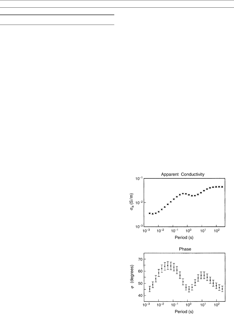
An apparent resistivity and phase can be defined in terms of the

impedance:

ðoÞ¼ðom

1

jZðoÞj

fðoÞ¼a tanðZðoÞÞ: (Eq. 3)

If conductivity is independent of depth ðsðzÞsÞ then r

ðoÞs

1

and fðoÞp=2. In this case computation of the conductivity from

the measured impedance is trivial. For the realistic case where conduc-

tivity varies with depth, the apparent conductivity ðs

¼ r

1

Þ is a

function of frequency (Figure E6). Conversion from apparent conduc-

tivity as a function of frequency ðs

ðoÞÞ to actual conductivity as a

function of depth ðsðzÞÞ is the essence of the 1D EM inverse problem

(Figures E6 and E7).

Exact measurements of ZðoÞ at an infinite number of frequencies

determines sðzÞ uniquely. However, as with all practical inverse pro-

blems, real data are finite in number and imprecise, so solutions to

the MT inverse problem are highly nonunique. In general, MT data

constrain only the product of conductivity and layer thickness (the

conductance), not the actual conductivity or layer thickness. Further-

more, the resolution of MT data tends to decrease with increasing

depth, and the actual resistivity of a section beneath a more conducting

layer is typically poorly determined.

A number of approaches for constructing specific solutions to the

inverse problem have been proposed. The simplest involve approxi-

mate functional transformations of c ðoÞ or ZðoÞ to sðzÞ. Although

Figure E6 Apparent conductivity (inverse of apparent resistivity),

and phase from a five layer 1D model (Figure E7). (After Whittall

and Oldenburg, 1992).

EM MODELING, INVERSE 219

not true inversions (the conductivity profiles generated do not gener-

ally reproduce the observed response functions), these transformations

provide reasonable rough estimates of conductivity profiles in many

situations, and their derivations provide physical insight into the

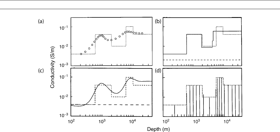
inverse problem. Perhaps the simplest example is the so-called

Schmucker inversion. Given cð o

Þ at a finite set of frequencies, define



¼<½cð o

Þ s



¼ð2 o

 1

=½ cð o

Þ

: (Eq. 4)

A plot of s



vs the discrete set of depths z



, can be shown to provide a

reasonable zero order approximation to the conductivity profile. An

example for the synthetic data of Figure E6 is given in Figure E7a.

Whittall and Oldenburg (1992) provide heuristic justification for

this simple approach, and describe a number of similar approximate

inversions.

More rigoro us inversion of MT data can be accomplished with stan-

dard methods of nonline ar geophysical inversion (e.g., Parker, 1994).

These methods can generally be formally reduced to minimization of

a penalty functional of the form

Jðm ; d Þ¼ðd  f ð m ÞÞ

 1

ð d  f ð mÞÞ

þðm  m

 1

ðm  m

Þ: (Eq. 5)

Here d is the data vector of dimension N

(e.g., real and imaginary

parts of the complex impedance Z ð o

Þ estimated at a discrete set of

frequencies), C

is the covariance matrix of data errors (typically diag-

onal), m is the N

-dimensional conductivity model parameter vector

(e.g., s

for a finite number of layers), f( m) defines the forward map-

ping, obtained by solving Eq. (1) at the appropriate frequency, m

a prior (or preferred) value of the conductivity parameter m , and C

is the covariance of the unknown model parameters used to regularize

the inversion (often given as a “ roughening operator ” C

1

Þ . The two

terms on the right-hand side of Eq. (5) penalize data misfit, and the norm

or size (in some general sense) of the model parameter m , respectively.

If the conductivity profile is described in terms of a small number

of parameters (e.g., 3 –5 layers of unknown thickness and conduc-

tivity, for a total of 6 –10 unknown parameters; see Figure E7b ), the

second term explicitly penalizing m is typically omitted. However,

frequently the conductivity model is overparameterized, with a large

number of thin layers of unknown conductivity. In this case there

are essentially an infinite number of parameter vectors that fit the

data equally well, so some sort of penalty on the model size (i.e.,

ð m  m

1

ð m  m

ÞÞ is required to make the problem well-

posed. Once the model parameterization and penalty functional are

defined, any of a number of standard search algorithms can be used

to seek the minimum of J . Some specific approaches are described

in Parker (1994). In general, these involve linearizing the forward

mappin g f (m ), though for the 1D inverse problem global Monte Carlo

search strategies which do not require explicit calculation of deriva-

tives, such as simulated annealing or the genetic algorithm, have been

successfully applied.

One very popular linearized approach is the “minimum structure ”

inversion. In this approach, the model penalty in Eq. (5) is the norm

of the first or second derivative of sð zÞ , and the minimizer of J is

the simplest (in the sense of flatness or smoothness of the conductivity

profile) consistent with the achieved data misfit ( Figure E7c). These

minimum structure models are less likely to contain features that are

not required by the data. Several different gradient-based optimization

algorithms have been used for minimum structure inversions; further

details can be found in Whittall and Oldenburg (1992) and Parker

(1994).

The 1D MT inverse problem is somewhat unusual in that a number

of exact nonlinear inversion algorithms are available. These are impor-

tant from a theoretical perspective since they provide a constructive

proof of existence and uniqueness of inverse solutions. However, these

exact nonlinear algorithms all require perfect and complete data, so

some adaptation is necessary to apply these to real finite noisy data

sets. Generally a two-step procedure is used (Whittall and Oldenburg,

1992): first the incomplete noisy data must be fit to a physically realiz-

able response at all frequencies; then the exact inversion is applied

to convert the completed response into the unique corresponding con-

ductivity profile. The most important example of this approach is the

so-called D

inversion of Parker (1980). Using the representation of

c ðo Þ in terms of the Sturm-Liouville spectrum of the differential

operator in Eq. (1) to complete the estimated response, Parker showed

that the best fitting conductivity model for real data sets would gen-

erally consist of a finite number of infinitely thin layers of finite

Figure E7 Examples of 1D inversions of the synthetic data of Figure E1. Dashed line gives actual layered model used to generate the

data. (a) Heuristic Schmucker inversion of Eq. (4). (b) Layered inversion, with the unknown structure defined by five layers of unknown

thickness and conductivity. (c) Minimum structure inversion, obtained by minimizing the norm of s

(z), subject to fitting the data within

error bars. (d) D

inversion, the model which best fits the synthetic data. Each line corresponds to a thin layer of finite conductance,

appropriately scaled to conductivity. (After Whittall and Oldenburg, 1992).

220 EM MODELING, INVERSE

conductance, separated by perfectly insulating layers of finite thick-

ness ( Figure E7d). Parker and Whaler (1981) developed a stable

numerical implementation of this inversion, which has since been

widely used in numerous practical applic ations. Although the conduc-

tivity profiles that result from this inversion are obviously not physi-

cally realistic, the D

inversion is very useful because it provides a

rigorous assessment of the degree to which a real data set is consistent

with the assumption of a 1D conductivity profile. The nature of the

best fitting profile is also instructive with regard to the nonuniqueness

of MT data: only conductan ce, and the rough distribution of conduc-

tance with depth, can be resolved by MT data, not the actual value

of conductivity at any depth (Figure E7).

Model apprai sal

Many particular conductivity profiles will fit any data set equall y

well, so assess ment of which features are common to all acceptable

solutions is an important part of the inverse problem. The classical

approach to model appraisal for linear problems is Backus-Gilbert the-

ory, based on construction of spatial averages of model parameters that

are constr ained by the data. For the nonlinear EM inverse problem this

resolution analysis requires linearization, and thus only provides a

rough characterization of nonuniqueness. Constrained inversion pro-

vides an alternative approach to inverse solution appraisal. For exam-

ple, to test if a particular conductive layer is require d, the inversion can

be run with conductivity in the appropriate depth range constrained to

a low value. If the data cannot be fit adequately subject to this con-

straint, but can be when the constraint is relaxed, higher conductivity

is required on average over this depth range. This general idea can

be formalized to construct upper and lower bounds on the total con-

ductance in a given depth range. Details of these, and related appraisal

methods for the 1D EM inverse problem are given in Whittall and

Oldenburg (1992).

Two- dimensi onal inversion

For 2D MT modeling a fixed geoelectric strike is assumed, with con-

ductivity sð y; zÞ varying across the strike ( y), and with depth (z ), but

not along the strike ( x). In this case the MT forward problem decou-

ples into two modes: the transverse electric (TE) or E-polarization mode,

with electric current s flowing only in the x-direction parallel to the geo-

logic structure, and the transverse magnetic (TM) or B-polarization

mode, with electric currents flowing only in the y-direction perpendicu-

lar to the strike. In both modes the horizontal magnetic fields are

still perpendicular to the electric fields, oriented across strike for TE,

and along strike for TM. Now there are distinct impedances for TE and

TM modes

¼ E

= H

; Z

¼ E

= H

; (Eq. 6)

as well as vertical field transfer functions (or “tippers ”) in the TE mode

T ¼ H

. As for the 1D case the impedances are often transformed

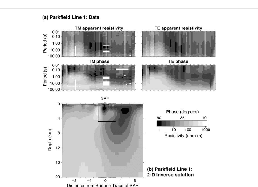
to apparent resistivities and phases, using Eq. (3). Data for 2D inter-

pretation are generally collected along a profile crossing the presumed

geoelectric strike. These data are commonly displayed as cross-strike

pseudosections, with frequency on the vertical axis (Figure E8). Conver-

sion of these images to conductivity sections, merging information from

both modes, and replacing frequency by depth, is the goal of 2D inver-

sion (Figure E8).

For the TE mode, Maxwe ll's equations can be reduced to a 2D

scalar diffusion equation for the along strike electric field

 iom

¼ 0: (Eq. 7)

This is analogous to the 1D equation of Eq. (1). For the TM mode,

Maxwell's equations can be reduced to a scalar equation in the along

strike magnetic field

þ s

1

rðsÞrðB

Þiom

¼ 0: (Eq. 8)

Discretizing Eqs. (7) and (8) with a finite-difference or finite-element

approximation results in systems of linear equations that can be solved

by a number of approaches, including forming and factoring the

banded coefficient matrix, and iterative Krylov space solvers such as

biconju gate gradients (e.g., Press et al., 1986).

Although existence and uniqueness of solutions to idealized 2D

inverse problems has been proven, theory is far less complete than

for the 1D case. In particular, there are no exact analytical procedures

for constructing inverse solutions to 2D problems, and there is no gen-

eral theory to establish consistency with a 2D interpretation for practi-

cal datasets.

Some approximate rapid schemes for converting 2D pseudosections

to conductivity images have been developed and used. These are

mostly based on rewriting the induction equations in integral form,

and then using a Born scattering approximation to reduce to an

approximate linear inverse problem. Although these methods can be

very fast, images constructed are not guaranteed to actually fit the data.

With increases in computing power, approaches based on minimizing

a penalty functional of the form (5) have become most popular. In

principle this can be accomplished with a straightforward extension

of the 1D methods, but with the 2D forward, Eqs. (7) and (8) replacing

Eq. (1) for computation of the forward mapping. However, for 2D pro-

blems there are many more unknown model parameters and data sets are

much larger, so issues of comput ational efficiency become much more

central.

Minimization of a penalty functional such as Eq. (5) is most directly

accomplished through some sort of gradient based search. The most

straightforwar d scheme is based on computing the Jacobian, i.e., the

 N

matrix of first derivatives of the forward mapping

G ¼

; (Eq. 9)

which can be accomplished most simply by solving nonhomogeneous

versions of Eqs. (7) and (8) for every frequency, for each of the N

column s of G . Using the fact that sources and receivers are symmetric

in the governing equations (“reciprocity”) computation of G can gen-

erally be accomplished more efficiently by solving one forward pro-

blem for each data point, with a source located at the data site. With

G available, the inverse problem can be linearized, and standard meth-

ods of linear inverse theory can be applied to find model parameters

which more closely fit the data. Using the updated model parameters,

G (which depends on the model conductivity) is recomputed and

the inverse model further refined. These steps are iterated until no

further reduction in J is possible. Details on several general schemes

for implementing such a linearized iterative search, including the most

commonly used for EM inverse problems, are given in Parker (1994),

Siripunvaraporn and Egbert (2000), and Rodi and Mackie (2001).

The reciprocity approach improves efficiency of the Jacobian com-

putations considerably, but construction and storage of G still requires

significant computer time and memory. A variety of computational

approaches have thus been proposed to make 2D inversion more prac-

tical. These include using approximations to the data sensitivities

based on simpler 1D models (Smith and Booker, 1991), and construct-

ing only a part of G to guide the linearized search (Siripunvaraporn

and Egbert, 2000). A very common approach used now is to directly

minimize J using a nonlinear conjugate gradient (NLCG) approach

(Press et al., 1986; Rodi and Mackie, 2001), completely avoiding con-

struction and storage of G. Each step in the NLCG search for the

(local) minimum requires computation of the gradient of J; this can

be shown to require two TE and TM forward solutions for each fre-

quency. NLCG is attractive because it completely avoids forming or

inverting large matrices. However, because many more iterations can

be required compared to schemes which make use of the Jacobian,

the number of forward solutions may not be significantly reduced,

EM MODELING, INVERSE 221

particularly in comparison with data space search schemes based on a

partial sensitivity computation (Siripunvaraporn and Egbert, 2000).

Nongradient based search schemes such as the genetic algorithm have

been tried for 2D EM inverse problems, but searching the compara-

tively large parameter space required to represent 2D conductivity var-

iations has not proven practical as yet.

Although a number of computationally feasible 2D MT inversion

schemes have been shown to perform quite well on synthetic data,

there are a number of complications with real data. Significant expert

user intervention is thus often still required for successful 2D inversion

of MT data. One challenging problem is that near surface small-scale

geology is often very complicated, and can almost never be repre-

sented by a single 2D model that matches the regional geoelectric

strike. Even if only superficial, these structures can galvanically distort

electric fields, resulting in frequency-independent “static shifts” of

apparent resistivity curves. Correction for these static shifts has been

found to be essential for correct interpretation of deeper structure. In

the context of inversion, additional model parameters are required to

account for these distortions. Estimation of these surface distortion

parameters has been integrated into some 2D inversion codes, but

separate distortion analysis is also generally now seen as a critical step

in 2D MT interpretation. Because phases are less effected by distortion

initial inversions of field data often emphasize fitting of phase data,

with apparent resistivities given less weight, and introduced later in a

multistage inversion sequence.

Deeper structure can also result in 3D complications. For example,

the EM response of a structure elongated along strike, but of finite

length, will depend on how close one is to the ends of the structure.

In general the TE mode, for which electric currents must flow through

the ends of the structure, is most severely effected. As such, TM

mode data are also often given higher weight, particularly for initial

stages of inversion. Regional structure may also pose difficulties for

2D inversion. For example, a nearby coastline may not be parallel to

the local geology. Since regional structure generally has a greater

influence at longer periods, this complication may be ameliorated by

emphasizing fit to shorter period data, but this of course limits the

depth of investigation.

A final, and very important potential complication in 2D interpreta-

tion is conductive anisotropy, which may well be ubiquitous in the

crust, and perhaps also the upper mantle. Allowing for conductivities

that depend on the direction of current flow significantly increases

the size of the model space, and as a result ambiguity and nonunique-

ness in EM inversions. Some 2D inversion codes now allow for aniso-

tropy, but there is so far little real understanding of resolution and

trade-offs when this richer model space is allowed for.

More generally, methods for model appraisal and characterization

of nonuniqueness in 2D EM inversion is an area of active research.

Linearized resolution analysis can be used if sensitivities are calcu-

lated, but the requirement of linearization is perhaps even more of a

limitation than for the 1D case. Testing for required features through

constrained inversion is also an option for 2D inversion, but methods

for constructing rigorous bounds on conductance that have been devel-

oped for the 1D EM inverse problem do not generalize in any obvious

way to higher dimension.

Figure E8 Example of a 2D MT data set and inversion. Pseudosections of (a) TE apparent resistivity; (b) TE phase; (c) TM apparent

resistivity; TM phase, from an MT survey near Parkfield California. (d) Resistivity section obtained by inversion of TE and TM data, using

a 2D minimum structure inversion. (After Siripunvaraporn and Egbert, 2000).

222 EM MODELING, INVERSE

Three-di mension al inver sion

Three-dimensional inversion is a natural extension of 2D inversion,

allowing for arbitrary variations of conductivity within the Earth. For

the 3D MT problem two possible source polarizations must be consid-

ered as in the 2D case, but now there is no preferred coordinate system

where the induction equations simplify or decouple. In the general 3D

case the MT impedance tensor (i.e., 2  2 frequency domain transfer

function matrix relating electric to magnetic fields at a site) has four

complex elements: Z

, Z

, along with a more general vertical

field transfer function giving local ratios of vertical to horizontal mag-

netic fields ( T

, T

). Mode l results for both polarizations are required to

form the impedance elements and transfer functions which can be fit in

the inversion. The forward problem generally involves solving a vector

diffusion equation, formulated variously in terms of electric or mag-

netic fields, or some sort of potentials. For example, in terms of the

3D vector electric fields E the forward problem can be expressed as

a PDE

rrE  i omsE ¼ 0 ; (Eq. 10)

which is to be solved subject to boundary conditions appropriate to the

source assumptions. Integral equation formulations are also used for

3D modeling and inversion. All formulations are readily derived from

the usual quasistatic approxim ation to Maxwell's equations. Factoring

the banded coefficient matrix obtained from a finite-difference or

finite-element discretization of Eq. (10) is practical for the analogous

2D problem, but prohibitively expensive in 3D. As a result the forward

3D problem is almost always solved with iterative techniques.

Few analytical results are available for the 3D EM inverse problem.

As for the 2D problem, efforts have focused on regularized inversion

through numerical minimization of a penalty functional such as

Eq. (5). Most of the discussion of 2D inversion methods is applicable

to the 3D case, but computational challenges are even greater. In par-

ticular, the number of model parameters is typically so large that stor-

ing the full Jacobian G is all but impossible. NLCG, which avoids

computing G altogether, is thus the most common approach to 3D

inversion. Other approaches which have had some success include

using very coarse parameterizations, and data space schemes which

avoid storing all of G.

As of this writing there is relatively little practical experience with

3D inversion. In addition to the severe computational challenges, there

are few data sets of sufficient density to truly resolve 3D structures.

Data sets collected in industry applications are the most extensive,

and much of the relevant experience with 3D inversion is in the private

sector, and with active source EM, often for near-surface applications.

Even with data sets that are not sufficiently extensive to truly image

3D structure, 3D inversion may be useful for obtaining more reliable

interpretations of profile data across approximately 2D structures.

Development of more efficient 3D inversion schemes, and learning

how to use these for interpretation of diverse EM data sets is an area

of active research.

Gary D. Egbert

Bibliography

Parker, R.L., 1980. The inverse problem of electromagnetic induction:

existence and construction of solutions based on incomplete data.

Journal of Geophysical Research, 85: 4421–4428.

Parker, R.L., and Whaler, K.A., 1981. Numerical methods for estab-

lishing solutions to the inverse problem of electromagnetic induc-

tion. Journal of Geophysical Research, 86: 9574–9584.

Parker, R.L., 1994. Geophysical Inverse Theory. Princeton, NJ:

Princeton University Press.

Press, W.H., Flanerrry, B.P., Teukolsky, S.A., and Vetterling, W.T.,

1986. Numerical Recipes: The Art of Scientific Computing. Cam-

bridge: Cambridge University Press.

Rodi, W.L., and Mackie, R.L., 2001. Nonlinear conjugate gradients

algorithm for 2-D magnetotelluric inversion. Geophysics, 66:

174–187.

Siripunvaraporn, W., and Egbert, G., 2000. An efficient data-subspace

inversion method for two-dimensional magnetotelluric data. Geo-

physics, 65: 791–803.

Smith, J.T., and Booker, J.R., 1991. Rapid inversion of two- and

three-dimensional magnetotelluric data. Journal of Geophysical

Research, 96: 3905–3922.

Whittall, K.P., and Oldenburg, D.W., 1992. Inversion of Magnetotelluric

Data for a One-Dimensional Conductivity. Geophysical Monograph

Series No. 5. Tulsa, OK: Society of Exploration Geophysicists.

Cross-references

Anisotropy, Electrical

Conductivity, Ocean Floor Measurements

EM Modeling, Forward

Galvanic Distortion

Geomagnetic Deep Sounding

Induction Arrows

Magnetotellurics

Robust Electromagnetic Transfer Functions Estimates

Transfer Functions

EM, INDUSTRIAL USES

Introduction

Mineral, petroleum, environmental, and geotechnical companies routi-

nely measure electrical conductivity properties of Earth materials to

map near-surface geological structures, locate economic resources,

and define environmental and engineering problems. Targets may be

more electrically conductive than the host environment, for example

in the case of many mineral deposits (Ohleoft, 1985) and for the location

of groundwater (McNeill, 1990). Alternatively, in the petroleum indus-

try the focus is often on regions that are less conductive than the host,

either in the case of a hydrocarbon-filled layer, or for an impermeable

formation such as salt domes that trap hydrocarbons (Hoverston et al.,

1998). For environmental and geotechnical studies, high-frequency

(>1 MHz) EM methods can also be used in a technique called

ground-penetrating radar (Daniels et al., 1988). At such high frequen-

cies, electrical conductivity is less important than the dielectric proper-

ties of the materials.

To measure the electrical conductivity, the primary methods are

either galvanic electrical techniques, in which a constant electrical cur-

rent is applied to the Earth, or EM induction techniques, in which elec-

trical currents are induced to flow in the Earth by a time-varying

external field. The external field can be either magnetic or electrical,

and the Earth's response is measured with a magnetometer (q.v.), an

electric dipole coupled to the ground, or a combination of both. The

time-varying signals originate either from natural sources, or applied,

controlled sources.

EM methods in common use by industry can be broadly categorized

in terms of the type of source fields. If the source of the externally

varying field is sufficiently distant from the location of measure-

ment, the source is approximately plane-wave, and is said to be one-

dimensional (varying in only one direction). On the other hand, if

the source and the measurement are close, then the source is said to

be three-dimensional (varying in all spatial dimensions). This latter

category can be further subdivided into techniques that use a continu-

ously varying controlled source field, usually in the form of a sine

wave, known as frequency-domain electromagnetics (FEM), and those

that require a source that abruptly switches on and off as a square

wave, known as time-domain electromagnetics (TEM) or transient

electromagnetic induction (q.v.).

EM, INDUSTRIAL USES 223

EM methods have been adapted by industries to a wide range

of environments. There is a rapidly growing marine EM (q.v.) indus-

trial sector (Chave et al., 1991; Constable et al., 1998) in which

the source field is either due to natural changes in Earth's magnetic

field or a transmitter is towed behind a ship, and seafloor electrical

and magnetic receivers measure the induced signals. Marine EM

measurements of the subseabed electrical conductivity are comple-

mentary to seismic methods, and help reduce the risk by identifying

more suitable drilling targets. Aircraft and helicopters have been mod-

ified to carry a wide range of EM sensors, often with a transmitter loop

between nose, wingtips, and tail, and with a secondary magnetic

receiver towed behind the aircraft (Palacky and West, 1991). Airborne

measurements have long been used in mineral exploration by rapid

imaging of electrically conductive basement structures, often through

many meters of overburden (weathered materials). More recently,

these techniques have become important in natural resource manage-

ment for mapping surface salinity and deeper saline aquifers. Drill-

hole EM techniques are widely used in the petroleum industry to

determine the electrical conductivity properties of the sequences

surrounding the borehole, and in mineral and environmental indus-

tries to image the extent of structures away from the borehole

(Dyck, 1991).

Plane wave source methods

The most common types of plane wave methods are known as VLF (very

low frequency), AMT (audio-magnetotellurics (q.v.)), and CSAMT

(controlled-source magnetotellurics (q.v.)). The VLF method uses a dis-

tant vertical electric dipole (denoted E

) that results from a time-varying

current in a long wire orientated vertically above the ground (McNeill

and Labson, 1991). Such electric field dipoles are developed as military

radio transmitters and operate in the 15–24 kHz range, and are used for

global-scale communication with submarines. There are many such

transmitters around the world, thus providing a VLF signal in most parts

of the globe.

The vertical flow of current generates horizontal magnetic field

(denoted B

and B

) components, each perpendicular to the direction

of propagation, and a small electric field (E

) in the direction of propa-

gation. When the electric field E

is incident on a boundary between

two materials of different conductivity, electric charges are induced

at the interface. This modifies E

to produce a “current channeling”

effect, which produces a secondary magnetic field that has an anoma-

lous vertical component B

. It is this component that is measured in a

VLF survey. It is also possible to measure the ratio of the amplitudes

of the horizontal electric and magnetic field components at the Earth's

surface to determine the apparent resistivity and phase in the same

manner as the magnetotelluric method (Becken and Pedersen, 2003).

The primary advantage of the VLF method is that as the source-field

is always present and predictable, the anomalous B

field can be mea-

sured quickly with a roving magnetometer to provide a surface map of

the electrical conductivity structures.

Mineral and petroleum exploration can be carried out using the

magnetotelluric (q.v.) method (Vozoff, 1991; Zonge and Hughes,

1991). To provide the highest resolution in the top few kilometers of

Earth, frequencies in the bandwidth 1 Hz to 20 kHz are used. At the

high-end of the bandwidth, these frequencies are in the audio range,

hence the name AMT. Source-fields are either naturally occurring

lightning strikes at equatorial latitudes (essentially a large vertical elec-

tric field E

as for the VLF method), or provided by a controlled-

source that consists of a distant applied electric or magnetic dipole

field. In the AMT or CSAMT method , horizontal and orthogonal com-

ponents of the electric (E

and E

) and magnetic (B

and B

) fields

are measured to yield an apparent resistivity and phase as a function

of frequency. Forward modeling (q.v.) and inverse modeling (q.v.)

provide a depth-dependent image of electrical conductivity. Lateral

coverage is slower than the VLF method due to the requirement of

measuring the electric fields with grounded electrodes.

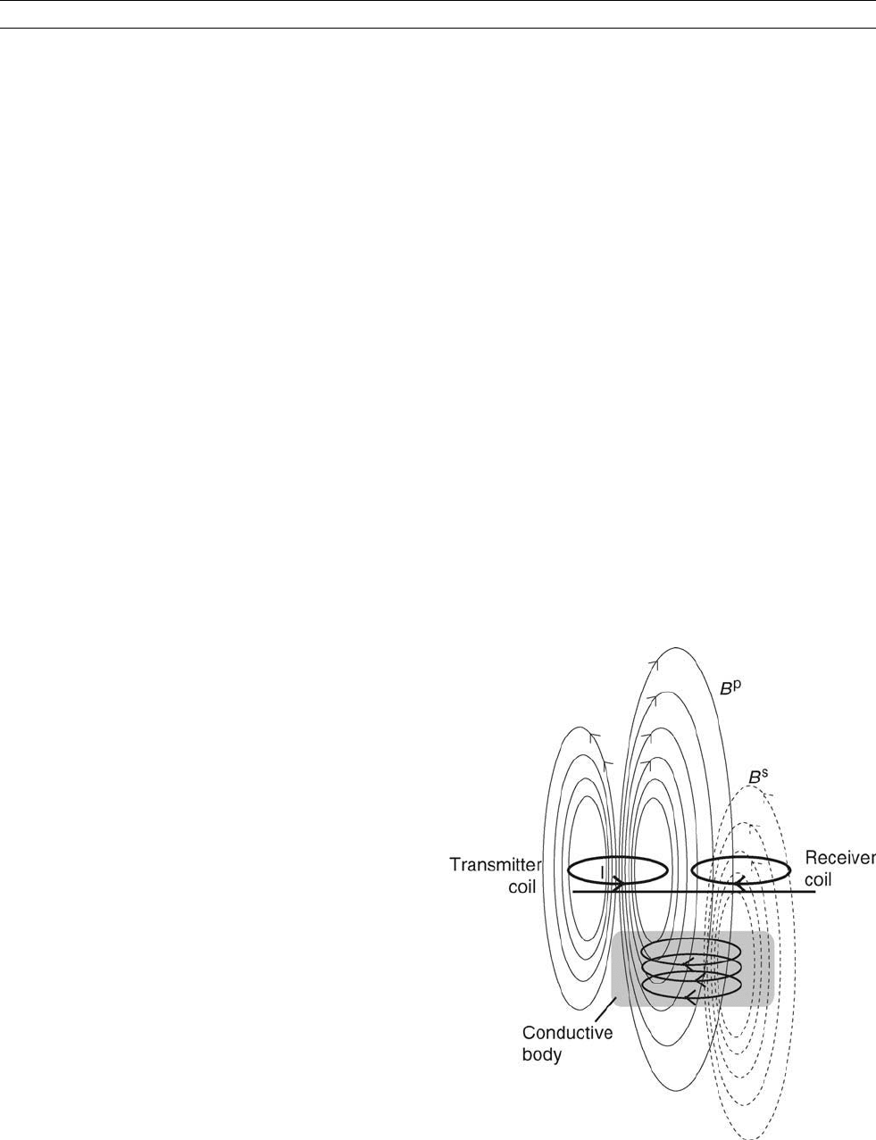
Frequency-domain electromagnetic (FEM) methods

In FEM methods, a time-varying current of a known frequency is applied

in a transmitter loop of wire at some location, as shown in Figure E9

(Frischknecht et al., 1991). The loop itself may consist of many turns

of wire. Electrical currents flowing in a loop generate a primary (p),

time-varying magnetic dipole field that will be horizontal (B

) if the loop

is orientated vertically, or vertical (B

) is the loop is flat on the ground.

The time-varying magnetic dipole fields induce eddy currents to flow

in Earth, which in turn generate secondary (s) magnetic fields B

,as

shown in Figure E10. A receiver at a nearby location, which can be a sec-

ond loop of wire, or a magnetometer (q.v.) sensor, measures a combina-

tion of the primary fields, B

, which is known, and the induced

secondary fields B

. The relative contribution of these fields depends

on the proximity and orientation of the receiver to the transmitter, and

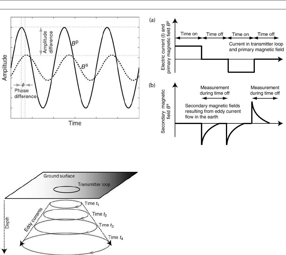
the electrical conductivity of the Earth between the two. The difference

in fields is usually measured as a combination of relative amplitude

and a phase difference, or as in-phase and out-of-phase (quadrature)

components.

In most commercial systems, measurements are made at one or

more frequencies, typically in the range 1–100 kHz. Variations in elec-

trical conductivity with depth can be determined by measurements

made at different frequencies, and by changing the orientation of the

coils. Lateral mapping can be achieved by moving either one or both

coils. Depth of penetration is relatively small, limited by the power

than can be produced by the transmitter.

FEM methods are widely used in environmental and geotechnical

studies, but are also becoming more widespread in marine EM (q.v.)

exploration for petroleum targets. A particularly common configura-

tion is known as a ground conductivity meter (McNeill, 1980), for

which the skin-depth of signal penetration is greater than the loop

separation. In this case, the quadrature (or out-of-phase) component

Figure E9 The arrangement of transmitter and receiver loops in

frequency-domain electromagnetic (FEM) systems. Current

flowing in the transmitter coil generates a primary magnetic (B

)

field that induces eddy currents in a conductor. The resulting

secondary magnetic fields (B

) are measured with a receiver loop.

224 EM, INDUSTRIAL USES

of the secondary field is linearly proportional to the ground apparent

resistivity, which allows rapid spatial mapping of electrical conductiv-

ity to be made by foot, vehicle, or helicopter.

Time-domain electromagnetic (TEM) methods

In TEM systems in Figures E11 and E12, the applied electric current in

a transmitter loop is switched on and off, in the form of a square wave

(Nabighian and Macnae, 1991). In the time intervals when the current

is on, a static primary magnetic field B

is established. When the trans-

mitter current in the loop is extinguished, the primary field collapses

almost instantly, and this rapid change in primary field generates large

eddy currents in the Earth, close to the surface. Such eddy currents in

turn yield a secondary magnetic field B

that can be measured with a

receiver loop, or a magnetometer sensor. Eddy currents continue to

flow after switch-off (typically for a few milliseconds) and become

broader and deeper. The resulting secondary magnetic field also

reduces in amplitude, in Figure E12. Energy is lost as heat, and the rate

of decay depends on the electrical conductivity of Earth.

TEM methods are widely used in the mineral exploration industry,

and are increasingly being used for environmental studies. There are

two significant advantages of TEM over FEM methods. Firstly, as

measurements of signals in the receiver loop or magnetometer sensor

need only be made in the intervals when the primary field is switched

off (i.e., B

¼ 0), it is easier to detect the small secondary field B

decay. Secondly, larger eddy currents can be induced as the primary

field changes much more rapidly than in FEM systems. The measured

decay in the secondary field can be converted to an apparent resistivity

as a function of time. Modeling and inversion techniques can then be

used to determine the electrical conductivity of Earth, typically as a

function of depth. TEM loops used in the minerals industry are often

of dimensions of hundreds of meters, with applied currents of tens of

amperes, to provide conductivity models to depth of several hundred

meters. For environmental studies the loops are typically 20 m, with

targets in the top 50 m.

Grounded wire methods

Methods that involve an injection of time-invariant electrical current

into the ground are generally denoted galvanic. Pathways, and result-

ing current densities, are determined by Earth's electrical conductivity,

and are typically measured as a horizontal electric field (E

and E

)by

a grounded dipole.

A variation on this approach is to measure the resulting secondary

magnetic field B

due to the subsurface current distribution (Edwards

et al., 1978; Edwards and Nabighian, 1991). The magnetometric resis-

tivity (MMR) technique is used in mineral exploration and has proved

to be useful in imaging basement structure beneath overburden. Two

advantages over traditional ground dipole measurements are that data

can be acquired rapidly as there is no requirement to have grounded

electrodes, and that the secondary magnetic field is the integral sum

of the contributions from all the current elements around the measure-

ment's location. The MMR method is therefore less sensitive to

near-surface inhomogeneities (Edwards, 1988).

Figure E10 The combination of primary (B

) and secondary (B

)

fields recorded with a FEM system. The measured response

can be determined in terms of an amplitude difference and/or

a phase difference f.

Figure E11 Distribution of eddy currents beneath a time-domain

transmitter. At time t

, immediately after switch-off, eddy

currents flow close to the surface; at progressively later times

to t

) eddy currents spread out and down.

Figure E12 Waveforms encountered in time domain EM

systems. (a) The top figure shows the applied current in the

transmitter loop and the resulting primary magnetic field.

(b) Secondary magnetic fields are measured in the times

when the current is switched off, and which are observed to

decay with time as eddy currents dissipate.

EM, INDUSTRIAL USES 225