Gubbins D., Herrero-Bervera E. Encyclopedia of Geomagnetism and Paleomagnetism

Подождите немного. Документ загружается.

DYNAMOS, FAST

As explained in other chapters dynamo action occurs when the effects

of advection (Faraday’s law) are vigorous enough to overcome the

effects of Ohmic diffusion. The ratio between these two effects is

expressed by the magnetic Reynolds number

UL=

where U, L are typical length and timescales, and  is the magnetic

diffusivity. If we nondimensionalize the induction equation by scaling

lengths with L and time with the turnover time L=U we get the follow-

ing form (assuming  uniform):

¼rðu  BÞR

1

rrB

At the onset of dynamo action, when induction just balances diffusion,

is of order unity by definition. However in some astrophysical

bodies (though probably not the Earth) R

is very large, and the ques-

tion then arises whether magnetic flux can grow at a rate Oð1Þ (that is

on the turnover time) or whether in fact the growth rate is much smal-

ler, depending on some negative power of R

(the rate R

1

would

imply growth on the Ohmic time L

=). If the first alternative holds,

we say that the dynamo is fast, otherwise it is slow.

It might be expected to be obvious from Faraday’s law (prohibiting

any change in the flux linked with a perfect conductor) that all dyna-

mos would be slow, since the growth rate at R

¼1would be zero.

However if as R

becomes very large the length scales of the magnetic

field become small, then diffusion can never be neglected, even in the

limit. Thus the question of the type of dynamo action is intimately

bound up with the complexity of the field structure.

It can be important to know whether the dynamo is fast or not; for

example the Ohmic time for the Sun is comparable with the age of

the universe, whereas the large-scale solar dynamo evolves on scales

of a few years. If the solar dynamo were not fast, then it would not

be able to generate flux in the way that it does.

While it is probably not the case that the Earth is in a regime appro-

priate for fast dynamo action, there is no doubt that our understanding

of dynamo action in general has been enhanced by the study of fast

dynamos, which have proved a valuable interface between MHD and

dynamical systems thory; see for example the monograph of Childress

and Gilbert (1995).

Examples of slow dynamos

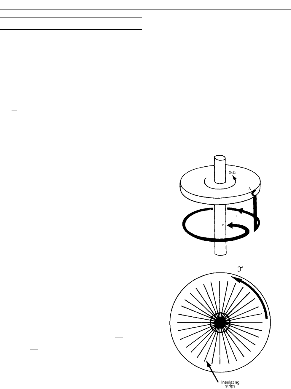
Here we give two rather different examples of slow dynamos. The first

is an adaptation of the Faraday disk dynamo introduced by Moffatt

(see Figure D23 and Dynamo, disk). Then there are simple equations

that relate current in the wire I, the current round the disk J, the

angular velocity O and the fluxes of magnetic field through the wire

and the disk F

; F

. These are

¼ LI þ MJ ; F

¼ MI þ L

J ; RI ¼ OF



;

J ¼

where M is the mutual inductance, and L; L

the self-inductances of the

circuit, and LL

> M

. We can seek solutions / e

, and find growth

(dynamo action) if oM > R. The growth rate is

ﬃﬃﬃﬃﬃﬃﬃﬃﬃﬃﬃﬃﬃﬃﬃﬃﬃﬃﬃﬃﬃﬃﬃﬃﬃﬃﬃﬃﬃﬃﬃﬃﬃﬃﬃﬃﬃﬃﬃﬃﬃﬃﬃﬃﬃﬃﬃﬃﬃﬃﬃﬃﬃﬃﬃﬃﬃﬃﬃﬃﬃﬃﬃﬃﬃﬃﬃﬃﬃﬃﬃﬃﬃﬃﬃﬃﬃﬃﬃﬃﬃ

ðRL

þ R

LÞ

þ 4R

ðOM  RÞðLL

 M



ðRL

þ R

LÞ



=2ðLL

 M

Þ:

> 0 for all O > R=M but p 

ﬃﬃﬃﬃﬃﬃﬃﬃ

as O !1. Identifying R

with  we can see that the growth rate scales as R

1=2

. This is not

really surprising since by Faraday’s law zero growth rate of the flux

through the disk should be expected as  !1.

A second slow dynamo is the so-called Roberts flow (Robert, 1970)

(see also Dynamos, periodic). This is a simple steady cellular flow

depending on only two space dimensions. The velocity takes the form

uðx; yÞ¼rðcðx; yÞe

Þþgcðx; yÞe

; c ¼ sin y þ cos x:

Thus we can see that the helicity hr  u  ui¼ghc

i. Solutions

exist in the form B ¼ Reð

Bðx; y; tÞe

ikz

Þ. The optimum growth rate

occurs at large k when R

 1, in fact ðk ðR

1=2

= ln R

Þ. These

scales, though small, are long compared to the thin boundary layer

scale R

1=2

for field near stagnation points. As R

!1the optimum

growth rate Oðlnðln R

Þ= ln R

Þ. This is just a slow dynamo! What

these two rather different examples have in common is that the flows

to not act to separate nearby points exponentially in time. That is, they

are not stretching flows (in fact the Roberts flow does have exponen-

tial stretching at the stagnation points of f, but nowhere else).

Figure D23 The segmented disk dynamo (Moffatt 1979). Radial

strips prevent circumferential current except in the outer part

of the disk.

186 DYNAMOS, FAST

Two examples of fast dynamos

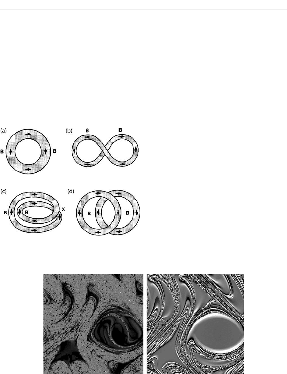
We now turn to two examples of fast dynamos. The first is the stretch-

twist-fold (STF) flow of Zel’dovich, which in the absence of

diffusion acts to double the magnetic energy by stretching. The dia-

gram in Figure D24 shows how the field has to be moved at large

, when the field lines are almost frozen in. Two issues immediately

arise. Firstly, the role of diffusion, however small, is not clear near the

cross-over points of the field, where gradients may be high. Secondly,

the flow field required is certainly not steady, or easily realizable in a

finite domain. However, it is possible to manufacture realistic flows

that have the required folding properties.

The second example is a development of the Roberts flow intro-

duced by Galloway and Proctor (1992). The velocity field (the

“GP-flow”) now takes the form: uðx; y; tÞ/rðcðx; y; tÞe

Þþ

gcðx; y; tÞ e

; c ¼ sinðy þ E sin otÞþcosðx þ E cos otÞ and it can be

seen that the Eulerian pattern of the Roberts flow is advected in a cir-

cle. However the Lagrangian pattern is completely different; while the

Roberts flow has no exponential separation of nearby points (except at

corners) the GP-flow has large stretching in large regions of the

domain. This can be seen by looking at the Liapunov exponents for

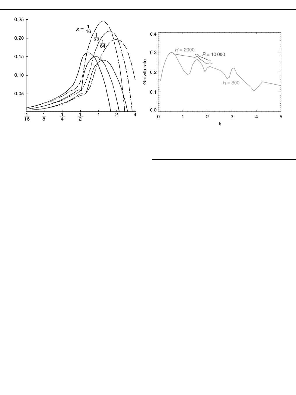
the flow with E ¼ o ¼ 1: The dynamo behavior of this flow is quite

different from that of the Roberts flow. For large R

, the growth rate

levels off at about 0.3, while the critical wavenumber converges to

about 0.57. The magnetic field structure becomes very complicated

in the limit of large R

, as can be seen in the right hand panel of

Figure D25. In fact diffusion remains important even in the limit,

and while the smallest scales  R

1=2

, the overall width of the flux

structures reaches a finite limit. The contrast between this behavior

and that of the Roberts flow can be seen in Figure D26. The key to this

complex behavior lies in a delicate balance between the stretching

properties of the flow, which tend to increase the energy at a rate

independent of diffusion, and the folding of flux elements back on

themselves which is inevitable given that the velocity does not lead

to unbounded excursions of fluid particles in general. If folding takes

place so as to bring oppositely directed field lines close together, the

resulting cancellation due to diffusion can result in a net decay of

the field. This always happens when the field is two-dimensional. In

three dimensions, however, with the right flow and the right scales

across the folding direction the folding can be constructive, leading

to net growth of the field even when diffusion is very small.

Nonlinear development

The idea of a fast dynamo is essentially a linear one, related to the rate

of growth of magnetic fields for a given velocity field u. If instead we

regard the velocity as being produced by some given force field, sub-

ject to the action of Lorentz forces, then as the field grows to finite

amplitude the flow field will be modified in such a way that the

growth of the field ceases. How is this achieved? One possibility is

that the vigor of the flow is decreased while its transport properties

remain constant; that is, equilibration is achieved by a reduction of

the effective R

. However, a number of numerical simulations of non-

linear dynamos suggest that instead reduction in dynamo action is

achieved by a change in the stretching properties of the flow, with little

change in the kinetic energy or other Eulerian properties. When there

is no significant field, the rate separation of fluid particles is uncon-

strained by their initial position. When there is a magnetic field pre-

sent, and R

is large on the dominant scales of the flow, then the

fluid particles are closely linked to the field lines and so acquire a

Figure D24 The STF dynamo (after Fearn et al., 1988). The initial

loop of flux is made to lie on top of itself but with twice the

original energy.

Figure D25 Left panel: Liapunov exponents for the GP-flow (courtesy of D.W. Hughes), found by integrating two nearby particle paths

for a finite time and measuring the total stretching; dark shades indicate small stretching, lighter shades higher stretching. Right panel:

intensity graph of the normal component of the dynamo field for this flow (courtesy of F. Cattaneo). Medium gray (red in online

encyclopedy) denotes weak, and white strong, field regions. Both plots show a periodic domain in the (x,y) plane. Note the close

correlation.

DYNAMOS, FAST 187

history; unlimited stretching is impossible without inducing large

Lorentz forces due to field line folding. When a stationary state is

reached the stretching is considerably reduced. The final velocity field

has less stretching than the linear flow, and is just such as to achieve a

zero growth rate. The resulting dynamo is thus neither slow nor fast,

just marginal!

Summary

By means of simple examples I have tried to demonstrate the distinc-

tion between fast and slow dynamos. From these it is clear that the

limit of infinite R

is not a simple one. Fast dynamos have become

the object of intense study by mathematicians: the outstanding mono-

graph describing this work, and much else concerning fast dynamos,

is that of Childress and Gilbert (1995). In the context of the geody-

namo, the limit of large R

is not approached, and the advection (turn-

over) time and the diffusion time can be considered comparable, so

that the limiting behavior discussed here is unlikely to be relevant.

Nonetheless, an understanding of dynamos at large R

has, as

explained above, proved very fruitful in advancing our understanding

of dynamos in general, including the geodynamo, and so an apprecia-

tion of the issues involved is very important.

Michael Proctor

Bibliography

Childress, S., and Gilbert, A.D., 1995. Stretch, Twist, Fold: The Fast

Dynamo. Berlin: Springer.

Fearn, D.R., Roberts, P.H., and Soward, A.M., 1988. Convection, sta-

bility and the dynamo. In Galdi, G.P., and Straughan, B. (ed),

Energy Stability and Convection. Pitman Research Notes in Mathe-

matics 168, pp. 60–324.

Galloway, D.J., and Proctor, M.R.E., 1992. Numerical calculations of

fast dynamos in smooth velocity fields. Nature, 356: 691–693.

Moffatt, H.K., 1979. A self-consistent treatment of simple dynamo

systems. Geophys. Astrophysical Fluid Dynamics, 14: 147–166.

Roberts, G.O., 1970. Spatially periodic dynamos. Philosophical Trans-

action of the Royal Society of London, A266: 535–558.

Cross-references

Dynamo, Disk

Dynamos, Periodic

DYNAMOS, KINEMATIC

Introduction

In the Earth’s fluid outer core, the motion of electrically conducting

molten iron is responsible for the generation of the magnetic field. In

general, this field reacts back onto the flow by the Lorentz force in a

nonlinear fashion, introducing complex behavior into the system

which is not well understood. Under the kinematic assumption, we

study the simpler problem in which the fluid flow is prescribed (and

typically time-independent), ignoring this back reaction. In this case,

we are at liberty to analyse the time behavior of the magnetic field

in isolation and test whether or not a given flow can act as a dynamo.

Such an analysis is a gross simplification, since the geodynamo is

thought to be in the so-called strong-field regime where the flow is

significantly affected by the magnetic field and will therefore differ

from any fixed kinematic flow structure. Such effects are taken into

account in fully dynamical models, however, these are so complex that

the behavior of the system often defies simplistic interpretation

(see Geodynamo, numerical simulations). Additionally, the parameter

values at which these models operate are so far from geophysical esti-

mates that it is by no means certain that the results can be extrapolated

to the Earth. Bearing this in mind, the analyses of simple kinematic

Earth-like models are important in the understanding of the dynamo

process.

The induction equation

The magnetic induction equation governs the time evolution of a mag-

netic field B under the influence of a moving conductor u (the outer

core) in the reference frame of the mantle and magnetic diffusion

(see Magnetohydrodynamics). It is written in nondimensional form

below, the sole parameter being the magnetic Reynolds number

¼UL=n where U is a typical value of the flow velocity, L is

the typical length scale taken to be the radius of the outer core and

 ¼ðm

sÞ

1

is the (constant) magnetic diffusivity, m

being the perme-

ability of free space, and s the electrical conductivity;

¼ R

rðu  BÞþr

B: (Eq. 1)

The value of R

is the ratio of the effects of the flow to magnetic

diffusion (associated with Ohmic dissipation of energy), and lies in

Figure D26 Left panel: Growth rates for the Roberts flow as a function of k for various R

¼ 1=e (solid lines, numerical results, dotted

lines, asymptotic theory); right panel: Growth rates as a function of k for the GP-flow.

188 DYNAMOS, KINEMATIC

the geophysical range of 500–1000. Time has been scaled relative to

the a priori magnetic diffusion timescale L

=n, which is typically

200000 years for the Earth. A straightforward analysis however shows

that the true diffusive decay time for the Earth is more like 20000

years (see Moffatt, 1978). The exterior of the outer core is the mantle,

well approximated by an electrical insulator (see Mantle, electrical

conductivity, mineralogy). The inner core is often ignored for simpli-

city, but if included, is given the same conductivity as the outer core.

Kinematic dynamo theory is concerned with magnetic field solu-

tions of Eq. (1) that grow in time given a flow structure u.Itisby

no means obvious that these exist, for in a sphere the dynamo mechan-

ism, associated with electric currents, could easily short-circuit prohi-

biting any magnetic field to grow. Nevertheless, growing solutions

have been found, as is outlined in the historical overview below. In

general, the kinematic assumption is valid assuming firstly we choose

a geophysically motivated flow, plausibly generated by rotating con-

vection (see Core convection) and secondly that the Lorentz force is

small, usually taken to mean that the initial and subsequent magnetic

fields are also small.

The induction equation is typically solved in a spherical geometry

using vector spherical harmonics (see Harmonics, spherical ), in which

the divergence-free magnetic field is expanded in toroidal-poloidal

form (see Moffatt, 1978).

The outer core is commonly taken to be incompressible and so u

may also be written in this way:

u ¼

l;m

þ s

l;m

r½Y

ðy; fÞt

ðrÞ

rþrr

½Y

ðy; fÞs

ðrÞ

r

ðEq: 2Þ

where l and m are the degree and order of the spherical harmonic

ðy; fÞ (in spherical polar coordinates), and

r is the unit position

vector. The toroidal and poloidal scalar functions t

and s

are given.

The magnetic field is written in a similar fashion as B ¼

l;m

þ S

(always using upper case). The value m ¼ 0 represents a vector inde-

pendent of f, axisymmetric about the z-axis.

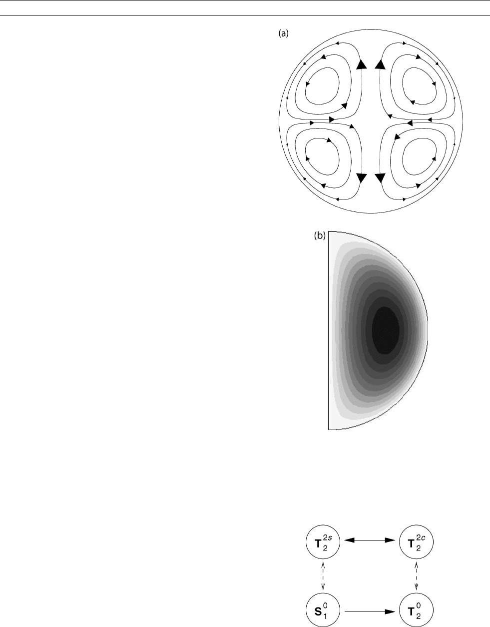
A typical flow comprises several harmonic components, for exam-

ple, t

representing differential rotation and s

representing convection

as shown in Figure D27, being nonslip at the boundary r ¼ 1. Both of

these components are important aspects of core convection.

An historica l overview: after Cowling’s theorem

Cowling’s theorem (q.v.), published in 1933, caused a major setback in

the early days of geodynamo theory. It proved that no axisymmetric

field could be sustained by dynamo action and since the Earth’s field

is principally of this type, it was thought at the time that the geody-

namo hypothesis was untenable. Indeed, it was not known whether a

general antidynamo theorem (see Antidynamo and bounding theorems)

might exist thus ruling out any kind of generative mechanism alto-

gether. In 1947 Elsasser (see Elsasser, Walter M.) was the first to

suggest that a complex mechanism might be taking place within the

outer core, converting magnetic field between symmetries thus break-

ing the constraints of Cowling’s theorem. He suggested that differen-

tial rotation could convert an axisymmetric dipole field, represented

by the S

vector harmonic, into T

by what is now called the o-effect

(see Dynamos, mean field).

The problem remained of how to close the loop, that is, how to

change the newly created T

field back into S

so that the process might

continue indefinitely. Of the two mechanisms he suggested, namely tur-

bulence and tilted flows, the latter was pursued by Bullard (see Bullard,

Edward Crisp) who argued qualitatively that a flow component s

(describing a tilted convection roll) might be sufficient to regenerate

the axial dipole field. Figure D28 shows a schematic picture of this pro-

cess. Solid arrows show the effect on the field of the t

flow; dashed

Figure D27 (a) Streamlines of an s

flow in a meridian plane;

(b) contours of u

in a meridian plane of a t

flow, giving rise to

differential rotation, the flow differing from solid body rotation

and is faster midstream than at the boundaries.

Figure D28 The interactions between the lowest degree

harmonics involving the axial dipole S

that forms a closed loop.

Solid arrows denote coupling by t

motion; dashed by s

. If all

links of this chain work sufficiently quickly then the axial dipole

harmonic could be infinitely sustained by this process.

DYNAMOS, KINEMATIC 189

arrows show the effect of the flow component s

. Thus, an S

field, if

acted upon in this manner, might be sustained creating byproducts of

, T

, and T

fields en route. The emphasis at this time was on find-

ing a mechanism whereby the principally observed geophysical field

component ðS

Þ could be sustained; no attention was given to other

field symmetries. Since this four component field is not axisymmetric,

Cowling’s theorem does not apply and the idea is plausible.

The Bullard and Gellman model

The first quantitative model of a self-sustaining process taking place

inside the Earth’s core was proposed by Takeuchi and Shimazu

(1953). This work was closely followed by Bullard and Gellman

(1954) (see Dynamo, Bullard-Gellman); both papers extended the sug-

gestions of Elsasser and Bullard that if a flow was chosen carefully,

through a sequence of interactions, the original field might be ampli-

fied and lead to a self-sustaining process.

The original procedure used to solve the induction equation was

to seek steady fields, which after numerical discretisation, converts

Eq. (1) into a generalized eigenvalue problem for R

; a steady solution

was manifested by the existence of a real eigenvalue. The magnetic

field was expanded in vector spherical harmonics and each unknown

radial scalar function using a finite difference scheme. The velocity

chosen was defined by

ðrÞ¼er

ð1  rÞ s

¼ r

ð1  rÞ

(Eq. 3)

where e is an adjustable parameter. No inner core was included in the

flow pattern to make it as simple as possible. Real eigenvalues were

found for R

, which did not appear to be affected greatly by changing

the numerical resolution, at least within the limited computer resources

available at that time. Thus it had appeared that a working dynamo had

been discovered: the combinations of the differential rotation t

and

the tilted convection roll s

was such that a (nonaxisymmetric) steady

field could be maintained with an Earth-like S

component. However,

13 years later, a repeat of the calculations (Gibson and Roberts, 1967)

at higher resolution using vastly more powerful computers showed that

the positive dynamo action found was spurious: the results were

merely an artifact of the inadequate numerical method used and not

of the underlying physics. The question of the possibility of dynamo

action in a homogeneous conducting sphere was again reopened.

Other advances

In 1958 both Backus (see Dynamo, Backus) and Herzenberg (see

Dynamo, Herzenberg) published analytic studies that strengthened

the belief that dynamo action was possible. The problem with the

induction effect is that for any length scale, successively smaller scales

will be created by the fluid-field interactions. Numerically it is hoped

that on increasing the resolution, the solution converges sufficiently

quickly to be captured with the available computing resources. Both

of these dynamos use diffusive effects to kill off the small-scale fields:

the Backus dynamo by periods of stasis and the Herzenberg dynamo

by spatial attenuation, both amenable in analytic treatment. Neither of

these solutions would be a possible candidate for the Earth; however,

this was evidence that no generalized antidynamo theorem existed.

The study of the dynamo problem in a sphere was also complimen-

ted by calculations in other geometries. An analytical solution of a

working dynamo in a cylindrical helical flow was published in 1973

by Ponomarenko (see Dynamo, Ponomarenko). Roberts (1970) studied

infinite spatially periodic dynamos, and found that almost all motions

performed as working dynamos. This was real evidence that not only

was it possible to find flows that worked as dynamos but that it was

relatively easy to do so, finally laying to rest the fear of a generalised

antidynamo theorem and gave dynamo theory centre stage for the ori-

gin of Earth’s magnetic field.

Further work on spherical dynamos

In the 1970s and onward, much progress was made with spherical

kinematic dynamos. Lilley (1970) studied the flow u ¼ t

þ s

and found ostensibly converged growing magnetic field solutions.

Unfortunately, yet again, later workers discovered his results to be

unconverged; this was to be the last of the spurious discoveries. The

first converged solutions were presented by Gubbins (1972), Roberts

(1972), and Pekeris et al. (1973). The method of solution had switched

from seeking steady solutions (leading to a generalised eigenvalue pro-

blem for R

) to time-dependent eigenmode solutions. In this paradigm,

the assumption that B ¼

is made thereby reducing the induction

equation to an eigenvalue problem for the complex growth rate l.

The adjustable parameter R

was varied and the lowest value giving

<ðlÞ¼0 sought. If such a value could be found (which was by no

means certain) this was termed the critical magnetic Reynolds number

ðR

Þ. It is entirely possible that =ðlÞ 6¼ 0 in this critical state so that

the dynamo would be oscillatory.

In the various flows studied, these workers found growing magnetic

fields although not always of the correct symmetry for the Earth.

Nonetheless, this was the first concrete evidence that the geodynamo

could work, at least in a simplified case. It was also found that a

greater flow complexity introduced by the choice of radial scalar func-

tions favoured dynamo action, i.e., the critical value of R

was smaller.

This characteristic was also found in the study of the nonaxisymmetric

flow of Kumar and Roberts (1975) with four components:

u ¼ t

þ e

(Eq. 4)

where the values of e

; e

, and e

are adjustable. The t

component

again represented an azimuthal differential rotation, the s

a meridional

circulation, and the s

and s

terms tilted convection rolls. They

found converged field solutions containing the axial dipole, and that

the direction of the flow components (i.e., the sign of the values of

) was crucial in determining the symmetry of the growing magnetic

field.

In later studies of the Kumar and Roberts flow (e.g., Sarson and

Gubbins, 1996; Gubbins et al., 2000) it was found that steady mag-

netic field solutions were favored with strong meridional circulation.

The inclusion of a solid inner core introduced significant changes in

the field solutions; the fact that different symmetries adapted in differ-

ent ways led to the possibility that the inner core might play a role in

field symmetry selection. Additionally, it was concluded that whether

or not kinematic dynamo action exists depends critically on the exact

choice of flow, an issue that makes it difficult to attribute a robust phy-

sical interpretation to such a dynamo mechanism. The influence of

helicity (the spiralling nature of the flow) was found to be favourable

to dynamo action, although was not essential.

Despite the correlation between increasing flow spatial complexity

and dynamo efficiency, Dudley and James (1989) found growing mag-

netic field solutions in very simple axisymmetric convection roll

flows, of t

; t

, and t

type. The fact that a one cell convective

flow t

can support dynamo action dispelled beliefs that the flow

had to be complex in nature, as previous results suggested.

An alternative methodology to solving the kinematic dynamo pro-

blem, instead of seeking eigenvalue solutions as has been popular

in most of the previous literature, is to apply an energetic analysis

(Livermore and Jackson, 2004). Under this paradigm, instead of only

seeking exponentially indefinitely growing solutions, any magnetic

field that grows is sought, including those that eventually decay. Cru-

cially, they found that the dynamo action, although not necessarily

indefinite, was robust under small changes in the flow, something that

previous studies did not find. It is therefore much more straightforward

to assign a physical mechanism to such a dynamo process, in this case

attributable to magnetic field line stretching by upwelling convective

flows, generating Earth-like S

fields.

190 DYNAMOS, KINEMATIC

The influence of an insulating boundary

Despite many authors finding spherical flows that operated as kine-

matic dynamos, it was well known that many other choices failed. This

was in stark constrast to Roberts (1970) who had showed that almost

all infinite spatially periodic flows show dynamo action. One cause

has been attributed to the influence of the mantle, introducing electri-

cally insulating boundary conditions on the magnetic field, these

making no appearance in a periodic domain. The study of Bullard

and Gubbins (1977) showed that the insulating boundary trapped cur-

rents near the edge of the flow region and catastrophically increased

Ohmic dissipation, inhibiting dynamo action. They suggested that this

might not be a problem if the flow near the CMB was quiescent, a

topic later taken up by Hutchenson and Gubbins (1994). They found

that the addition of a static outer conducting region on top of the fluid

core promoted dynamo action: either the critical magnetic Reynolds

number was lowered or growing magnetic fields were found when

all had previously decayed. The trapped currents could now flow out-

side the core region facilitating dynamo action, geophysically moti-

vated by the possibility of a stably stratified layer at the top of the

outer core.

Motivating the choice of flow

Although one of the great strengths of kinematic theory is the ability to

prescribe the flow, the lack of physical self-consistency is one of its

great drawbacks. To partially mitigate this issue, Love and Gubbins

(1996) studied the problem whereby the dynamo efficiency, defined

in terms of the critical magnetic Reynolds number and the Ohmic dis-

sipation produced by the growing field, was minimized over a choice

of flow (in this case the the values of e in the Kumar and Roberts

flow). Such a method of choosing a flow has a strong basis on physical

grounds because it might be energetically favored. They found

dynamo action with much reduced Ohmic dissipation.

A partial solution to the full Navier-Stokes equations (see Geody-

namo) is another way of choosing the flow. Sarson (2003) considered

the geophysically relevant geostrophic approximation, balancing the

Coriolis force, buoyancy, and pressure. He derived a fully consistent

flow although the driving temperature profile was not geophysically

plausible, and found growing field solutions of dipole symmetry in

line with the studies of the Kumar and Roberts flow.

Summary

Kinematic dynamo theory has proven very successful in helping scien-

tists understand the complex process of magnetic field generation

inside the Earth. Conclusive evidence in the 1970s that the geodynamo

could function is of particular historical importance and paved the way

for many of the subsequent advances in geodynamo theory. In addi-

tion, some links have been made between the generated fields and var-

ious flow properties and the presence of a thin stably stratified

conducting layer on top of the outer core. Kinematic reversal mechan-

isms have also been proposed (see Reversals, theory).

The main outstanding problem of kinematic dynamos is their sensi-

tivity to the exact choice of flow chosen, making it difficult to attribute

physical processes in such cases. Nevertheless, complex dynamical

models are still often understood by simple kinematic arguments and

this will undoubtedly remain the case for the foreseeable future.

Philip W. Livermore

Bibliography

Bullard, E., and Gellman, H., 1954. Homogeneous dynamos and ter-

restrial magnetism, Philosophical Transactions of the Royal

Society of London A, 247: 213–278.

Bullard, E., and Gubbins D., 1977. Generation of magnetic fields by

fluid motions of global scale. Geophysical and Astrophysical Fluid

Dynamics, 8:43–56.

Dudley, M., and James R., 1989. Time‐dependent kinematic dynamos

with stationary flows. Proceedings of the Royal Society of London

A, 425: 407–429.

Gibson, R., and Roberts, P., 1967. Some comments on the theory of

homogeneous dynamos. In Hindmarsh et al. (ed.), Magnetism

and the Cosmos. Oliver and Boyd, pp. 108–120.

Gubbins, D., 1973. Numerical solutions of the kinematic dynamo pro-

blem. Philosophical Transactions of the Royal Society of London

A, 274: 493–521.

Gubbins, D. et al., 2000. Kinematic dynamo action in a sphere: I.

Effects of differential rotation and meridional circulation on solu-

tions with axial dipole symmetry. Proceedings of the Royal Society

of London A, 456: 1333–1353.

Hutchenson, K., and Gubbins, D., 1994. Kinematic magnetic‐field

morphology at the core‐ mantle boundary. Geophysical Journal

International, 116: 304–320.

Kumar, S., and Roberts, P., 1975. A three‐dimensional dynamo

problem. Proceedings of the Royal Society of London A, 344:

235–258.

Lilley, F., 1970. On kinematic dynamos. Proceedings of the Royal

Society of London A, 316: 153–167.

Livermore, P., and Jackson, A., 2004. On magnetic energy instability

in spherical stationary flows. Proceedings of the Royal Society of

London A. In press.

Love, J., and Gubbins, D., 1996. Optimized Kinematic Dynamos.

Geophysical Journal International, 124: 787

–800.

Moffatt, H., 1978. Magnetic field generation in electrically conducting

fluids. Cambridge University Press.

Pekeris, C. et al., 1973. Kinematic dynamos and the Earth's magnetic

field. Philosophical Transactions of the Royal Society of London A,

275: 425–461.

Roberts, G., 1970. Spatially periodic dynamos. Philosophical Transac-

tions of the Royal Society of London A, 266: 535–558.

Roberts, P., 1972. Kinematic dynamo models. Philosophical Transac-

tions of the Royal Society of London A, 272: 663–698.

Sarson, G., 2003. Kinematic dynamos driven by thermal wind flows.

Proceedings of the Royal Society of London A, 459: 1241–1259.

Sarson, G., and Gubbins, D., 1996. Three‐dimensional kinematic

dynamos dominated by strong differential rotation. Journal of

Fluid Mechanics, 306: 223–265.

Takeuchi, H., and Shimazu, Y., 1953. On a self‐exciting process in

magneto‐hydrodynamics. Journal of Geophysical Research, 58:

497–518.

Cross-references

Antidynamo and Bounding Theorems

Bullard, Edward Crisp (1907–1980)

Core Convection

Cowling’s Theorem

Dynamo, Backus

Dynamo, Bullard-Gellman

Dynamo, Herzenberg

Dynamo, Ponomarenko

Dynamos, Mean Field

Elsasser, Walter M. (1904–1991)

Geodynamo

Geodynamo, Numerical Simulations

Harmonics, Spherical

Magnetohydrodynamics

Mantle, Electrical Conductivity, Mineralogy

Reversals, Theory

DYNAMOS, KINEMATIC 191

DYNAMOS, MEAN-FIELD

Intro ductio n

The mean-field concept was introduced into the dynamo theory of the

magnetic fields of the Earth, the Sun, and other cosmic objects in the

sixties of the last century. As was known or at least considered as very

probable at that time, magnetic fields as well as the motions inside the

electrically conducting interiors of these objects show rather complex

geometrical structures and time behaviors. In addition antidynamo the-

orems suggested that dynamo action requires a certain complexity of

magnetic field and motion (see Antidynamo theorems or Cowling ’s

theorem ). No solution of the dynamo equations has been found until

this time, which could be interpreted as an approximate picture of

the situation in the Earth or any cosmic body.

The central idea of the mean-field concept is to define mean magnetic

fields, mean veloci ty fields etc., which reflect essential features of the

original fields but show simpler, that is more smooth, geometrical struc-

tures and time behaviors, and to derive equati ons for them, which are

easily treatable, in particular numerically solvable with the available

tools. Of course, these equations must contain terms accounting for

the deviations of the original fields from the mean fields, in which these

deviations, however, enter only in the form of averaged quantities.

On the basis of this concept indeed dynamo models for the Earth,

the Sun, and many other cosmic objects including galaxies have been

developed. A remarkable step in this direction was done by Braginsky

in 1964, who considered the Earth and proposed the theory of the

“nearly symmetric dynamo” (Braginsky, 1964a,b) (see Dynamo,

Braginsky and Dynamo, model Z). Independent from this, a general

mean-field electrodynamics was established by Steenbeck et al. in

1966, and it was used to develop a general mean-field dynamo theory,

applicable to all objects mentioned (Steenbeck et al., 1966; Krause

et al ., 1980). The rigorous mathematical formulation of the mean-field

theory also covers Parker’s ideas on dynamo action described already

in 1955 (Parker, 1955, 1957).

A crucial point in mean-field electrodynamics and mean-field

dynamo theory is a mean electromotive force resulting from the devia-

tions of motion and magnetic field from mean motion and mean mag-

netic field. The occurrence of a specific type of this electromotive

force, with a component in the direction of the mean magnetic field,

is called “ a -effect” . The mean-field dynamo theory revealed basic

dynamo mechanisms working with the a -effect or with related effects.

In this way it created a system of ideas which is now of importance in

all dynamo theory, also beyond the mean-field theory.

As far as the geodynamo is concerned, a series of direct numerical

simulations on very powerful computers has been carried out since the

end of the last century (see Geodynamo, numerical simulations). The

mean-field dynamo models, which, although in some respect problematic,

were important for designing the more advanced models investigated

in this way, are now no longer of primary interest. Nevertheless, the

mean-field concept is still a useful tool for the interpretation of the

numerical results and for understanding the basic dynamo mechanisms.

In view of the solar and other cosmical dynamos, however, the mean-

field approa ch is till now the only adequate way of describing and

investigating them.

In this article a brief outline is given of the main ideas of mean-field

electrodynamics and the dynamo theory based on it as well as a few

specific applications to the geodynamo. See also more detailed presen-

tations (e.g., Moffatt, 1978; Krause et al., 1980; Zeldovich et al., 1983;

Rädler, 1995, 2000).

Mean- field electro dynamics

Basic equation s

The standard dynamo theory assumes that the electromagnetic field in

an electrically conducting moving fluid is governed by the Maxwell

equations and Ohm’s law in the form

rE ¼]

B ;rB ¼ m j ;r B ¼ 0 (Eq. 1)

j ¼ sð E þ u  B Þ: (Eq. 2)

As usual, E is the electric field and B the magnetic flux density, simply

called magnetic field in the following, j is the electric current density,

u the velocity of the fluid motion, m the magnetic permeability of the

fluid, assumed to be equal to that of free space, and s the electric conduc-

tivity of the fluid. These equations together with proper initial and

boundary conditions determine B, E, and j if u is given. They can be

reduced to the induction equation for B alone. For the sake of simplicity

it is assumed here that s does not vary in space. Then it follows that

r

B þrðu  B Þ]

B ¼ 0 ;r B ¼ 0 ; (Eq. 3)

where  is the magnetic diffusivity defined by ¼ 1 =ms.IfB is

known from these equations for a given u, then both E and j can be

determined without further integrations.

Def inition of mean fields

Let us focus our attention on situations in which the fluid motion

possess es components showing spatial scales that are small compared

to the scales of fluid body considered. Typical examples of that are

turbulent or convective motions. Then, of course, the electromagnetic

field has to show small scales in that sense, too.

In view of the definition of mean fields we consider first a scalar field

F. We define the corresponding mean field

F as an average of F

obtained with an averaging procedure which, as a rule, smoothes its

variations in space and time. Adopting the terminology of turbulence

theory the difference F

¼ F  F is called “ fluctuation. ” To extend

the definition to a vector field F we refer to a coordinate system with

unit vectors e

ð iÞ

and write, using the summation convention,

F ¼ e

ðiÞ

. Then we define the mean-field F by F ¼ e

ðiÞ

Various choices of the averaging procedure may be admitted. The

only requirement is that Reynolds ’ averaging rules apply exactly or

at least as an approximation. They read

F þ G ¼ F þ G (Eq. 4)

] F =] x ¼ ]F = ]x ; ]F =] t ¼ ]F = ] t (Eq. 5)

F ¼ F or ; what is in this context the same ; F

¼ 0 (Eq. 6)

FG ¼ F G ; (Eq. 7)

where F as well as G are arbitrary fields, and x stands for any space

coordinate. Clearly Eq. (6) is a special case of Eq. (7). An important

consequence of Eqs. (4) and (7) is

FG ¼ F G þ F

As can easily be seen below, mean vector fields defined on the basis

of a Cartesian coordinate system are well different from those defined,

e.g., with respect to a cylindrical or a spherical coordinate system.

Giving now a few examples of averages we distinguish between

“local” averages, for which

F in a given point depends only on the

values of F in this point or a small neighborhood of it, and “nonlocal”

averages.

(i) Local averages

(ia) Statistical or ensemble averages. In this case we suppose that

there is an infinity of copies of the object considered. The individual

copies are labeled by a parameter, say p. In that sense any quantity F

192 DYNAMOS, MEAN-FIELD

to be avera ged depends, in addition to the space and time variables, x and

t, on this parameter p . The average

F ð x ; t Þ is then defined by averaging F

over all p . Averages of this kind clearly ensure the validity of all four

rules Eqs. (4) –(7). There is, however, a serious difficulty to relate these

averages to observable quantities.

(ib) Space averages. A general form of a space average is given by

F ð x ; t Þ¼

F ðx þ j ; t Þg ðj Þ d

x ;

g ð j Þ d

x ¼ 1: (Eq. 8)

Here g ðj Þ is a normalized weight function which is different from zero

only in some region around j ¼ 0 . The integrations, formally over all

j -space, are in fact over this region only. With such averages the two

rules Eqs. (4) and (5) apply exactly but in general Eqs. (6) and (7) are

violated. The latter two can be justified as an approximation if there is

a gap in the spectrum of the length scales of F, and all large scales are

much larger, and all small ones much smaller than the characteristic

length of the averaging region. A situation of that kind is sometimes

named a “ two-scale situation ”.

(ic) Time averages. Similar to space averages, we may define time

averages by

F ð x ; t Þ¼

F ðx ; t þ tÞ g ðt Þ dt ;

g ð tÞ dt ¼ 1; (Eq. 9)

with some normalized weight function g ð tÞ diff eren t from z er o i n s om e

neighborhood of t ¼ 0. The comments made under (ib) apply analogously.

(ii) Nonl ocal averag es

(iia) Azimuthal average . There are, however, particular space averages

to which all averaging rules apply. Consider, for example, a case in

which the variation of F in space is properly described by spherical

coordinates r ; y ; j , and put

F ð r ; y ; t Þ¼

2 p

F ðr ; y ; j ; t Þ d j : (Eq. 10)

This kind of average is used in particular in Braginsky ’s theory of the

nearly symmetric dynamo. Of course, all mean-fields are by definition

axisymmetric. All four rules Eqs. (4)– (7) apply exactly.

(iib) Averages based on filtering of spectra . We may, for example,

represent F in its dependence on space coordinates by a Fourier integral

and define

F by another integral of this type which covers only the large-

scale part of the Fourier spectrum beyond some averaging scale. For

averages defined in this way the three rules Eqs. (4)– (6) apply exactly,

and with a sufficiently large gap in the spectrum and a proper choice of

the averaging scale the remaining rule Eq. (7) can again be justified as

an approximation. The azimuthal average defined by Eq. (10) can also

be interpreted as one based on filtering a Fourier spectrum with respect

to j. Another interesting possibility consists, e.g., in filtering the multi-

pole spectrum of vector fields so that the mean fields are just dipole

fields, or dipole and quadrupole fields, etc.

Basic mean-fiel d equ ations

Returning to the Eqs. (1),(2 ), and ( 3), we understand now B, E , j,

and u as superpositions of mean and fluctuating parts. Applying the

averaging procedure to Eqs. (1) and (2) we obtain

r

E ¼]

B ;rB ¼ m j ;rB ¼ 0 (Eq. 11)

j ¼ sðE þ u  B þ E Þ: (Eq. 12)

From these equations, or taking the average of Eq. (3), we further obtain

r

B þrðu  B þ E Þ ]

B ¼ 0 ;rB ¼ 0 : (Eq. 13)

E is the mean electromotive force due to the fluctuations of motion and

magnetic field,

E ¼

 B

: (Eq. 14)

These equations together with proper initial and boundary conditions

determine

B if u and E are given, and so also E and j .

The crucial point in the elaboration of mean-field electrodynamics is

the determination of the mean electromotive force E for given

u , u

and

B. Using Eqs. (3) and (13) , a n equation f or the magnetic fluctuations

can be derived. It allows us to conclude that B

can be considered as

a functional of

u, u

, and B, which is linear in B . Thus, E must show

the same dependence on these fields. For the sake of simplicity we

restrict our attention to the case in which the magnetic fluctuations

are due to the interaction of the velocity fluctuations u

with the

mean magnetic field

B only, that is, decay to zero if B is zero. In other

words, the possibility of a magnetohydrodynamic turbulence with zero

B is ignored. Apart from some initial time, which is not considered

here, E is then not only linear but also homogeneous in

B, that is,

has to vanish if

B does so. For the sake of simplicity we restrict our

attention first to mean fields defined by local averages. Then it can

be easily concluded that E allows the representation

ð x ; t Þ¼

ð x; t ; j ; tÞB

ðx þ j ; t  t Þ d

x d t; (Eq. 15)

with some kernel K

determined by u and u

. Here, and in what

follows, indices like i and j refer to a Cartesian coordinate system

and the summation convention is adopted.

Let us accept the further assumption that E in a given point in space

and time depends only on the values of u, u

, and B in some neighbor-

hood of this point. This can easily be justified in the case of turbulent

fluid motions but applies for most of the other situations of interest,

too. Let us assume further that the variations of

B in space and time

are weak enough so that its behavior in the relevant neighborhood of

the considered point is to a good approximation determined by

and its first spatial derivatives at this point. This implies that E can

be represented in the form

¼ a

þ b

ijk

= ] x

; (Eq. 16)

where the tensors a

and b

ijk

are mean quantities which are determined

u and u

but do not depend on B . It remains of course to be checked

in all applications that higher spatial derivatives or the time derivatives

B are indeed negligible. Incidentally, as a consequence of

r

B ¼ 0, three elements of b

ijk

can be arbitrarily fixed.

In the case of a nonlocal, e.g., the azimuthal average in Eqs. (15)

and (16) occur primarily in slightly different forms. We may, however,

justify Eq. (16) as well.

Let us consider the simple (somewhat academic) example in which

the mean motion is zero,

u ¼ 0, and the fluctuations of the velocity

field, u

, correspond to a homogeneous isotropic turbulence. In this

case, no preferred points in space and no preferred directions can be

found in the u

field. In other words, all mean quantities depending

on u

are invariant under arbitrary translations of the u

field and under

arbitrary rotations of this field about arbitrary axes. Simple symmetry

consideratio ns allow us then to conclude that a

and b

ijk

are isotropic

tensors and are independent on position. That is, a

¼ ad

and

ijk

¼ be

ijk

, where the coefficients a and b are independent of position

and determined by u

only, and d

and E

ijk

are the Kronecker and the

Levi-Civita tensors. This result allows us to write Eq. (16) in the form

DYNAMOS, MEAN-FIELD 193

E ¼ aB  b rB : (Eq. 17)

Together with Eqs. (11) and (12) this yields

j ¼ s

ðE þ aBÞ; s

1 þ b =

: (Eq. 18)

That is, in Ohm ’s law for the mean fields occurs a mean-field conduc-

tivity s

, which (if b 6¼ 0) differs from the molecular conductivity s.

In addition, there is (if a 6¼ 0) an electromotive force parallel (or anti-

parallel) to

B . This is remarkable as in the original form (Eq. (2)) of

Ohm’s law the magnetic field enters only via the term u  B , which

has no component in the direction of B . The occurrence of a mean

electromotive force with a component in the direction of the mean

magnetic field

B is called “a -effect. ”

The a-effect makes a dynamo possible. As can be easily followed

up, Eq. (13) for

B with u ¼ 0 and E specified according to Eq. (17)

possesses growing solutio ns for proper choices of ; a , and b.

Under realistic circumstances an isotropic turbulence is also reflec-

tionally symmetric (“ mirror-symmetric ”) in the sense that there is no

preference of left-handed over right-handed helical motions or vice

versa . More precisely, all mean quantities are invariant under reflections

of the u

field, e.g., at the origin of the coordinate system, that is, under

exchanging u

ð x ; t Þ with  u

ð x ; t Þ . Symmetry considerations show

then a ¼ 0. Although in a sense unrealistic, the simple example under

discussion reveals the fundamental connection between the violation

of reflectional symmetry of the turbulence and the a -effect. The turbu-

lence on a rotating body is neither homogeneous nor isotropic. Apart

from the fact that reflectional symmetry in the above sense is anyway

not compatible with inhomogeneity or anisotropy, it is in particular

disturbed by the influence of the Coriolis force. Inhomogeneity and

the violation of reflectional symmetry due to the Coriolis force lead

again to an a -effect similar to that discussed here and, as a consequence,

to dynamo action.

Leaving this simple example and returning to arbitrar y

u and the

representation of E in the form (Eq. (16)) we give an alternative repre-

sentation of E . The tensor a

may be split into a symmetric and

an antisymmetric part, and the latter can be expressed by a vector.

Likewise the gradient tensor ]

= ] x

can be represented by its sym-

metric part and a vector, which proves to be proportional to r

B .

Considering these possibilities we may write

E ¼a 

B  g B  b ðrBÞd ðrBÞk ðrB Þ

ðsÞ

(Eq. 19)

Here a and b are symmetric second-rank tensors, g and d vectors,

and k is a third-r ank tensor, all being determined by

u and u

Further ð H

B Þ

ðsÞ

is the symmetric part of the gradient tensor of B ,

that is, ð H

B Þ

ðsÞ

¼ð1 =2 Þð]B

=] x

þ ]B

= ] x

Þ . Of course, k may be

assumed to be symmetric in the indices connecting it with ðH

B Þ

ð sÞ

and because r

B ¼ 0 three of its elements can be fixed arbitrarily.

Inserting E according to Eq. (19) into Ohm ’s law Eq. (12), we may

write the latter in the form

j ¼ s

ðE  a B þðu  gÞB  d ðH B Þ k ðrBÞ

ðs Þ

Þ:

(Eq. 20)

Here, s

is a conductivity tensor incorporating the b term of Eq. (19)

and being symmetric. Again, the mean electric current is no longer

determined by the molecular conductivity, and the relation between

mean current and mean electric field plus mean electromotive force is

in general anisotropic. The a term defines some generalization of the

a -effect discussed above, that is, an anisotropic a -effect. The g term cor-

responds to a transport of mean magnetic flux like that by a mean motion,

which occurs however even in the absence of any mean motion. Clearly

u  g is the effective velocity for the transport of mean flux. The d term

describes an induction effect, which was first found in the special case

in which d was proportional to an angular velocity V and has been called

“V  j -effect”. The k term is less easy to interpret. Analogous to the

notation a-effect, we speak of “b -effect”, “ d -effect” etc. when referring

to the induction effects described by the terms with b , d etc. in Eqs.

(19) or (20). By the way, we arrive at an alternative form of Ohm’s law

if we interpret s

as tensor incorporating both the b and d terms and can-

cel the last ones otherwise. Then, however, s

is no longer symmetric.

It is important to know the dependence of the quantities a; b ; g ; d ,

and k on the fluid motion, that is, on

u and u

. Unfortunately there is

no simple way to derive general results of that kind. A series of

extended calculations have been carried out using specific approxima-

tions. Often the “second-order correlation approximation ”, also called

the “first-order smoothing approximation ” , has been adopted, which,

roughly speaking, can be justified only for u

not too large.

Assume for the sake of simplicity that

u ¼ 0 and u

represents a tur-

bulence with a characteristic velocity u

, a correlation length l

, and a

correlation time t

. Define then the magnetic Reynolds number

¼ u

= , the Strouhal number S ¼ u

= l

, and the quantity

q ¼ l

= t

, Clearly q is the ratio of the characteristic time l

= for

electromagneti c processes in a region with the length scale l

to the

time t

. In the high-conductivity limit, defined by q  1, a sufficient

condition for the applicability of the second-order correlation approx-

imation reads S  1. In the low-conductivity limit, q  1, the corre-

sponding sufficient condition is R

 1.

As an example we give here results for a and b for the simple case

in which u

corresponds to a homogeneous isotropic turbulence. In the

high-conductivity limit, q  1, this approximation yields

a ¼

ð x; t ÞðH  u

ð x ; t  tÞÞ dt ;

b ¼

ðx ; t Þ u

ð x ; t  tÞ d t; (Eq. 21)

a ¼

ðH  u

Þ t

ða Þ

; b ¼

0 2

ðb Þ

: (Eq. 22)

Here t

ða Þ

and t

ðb Þ

are primarily defined by equating the corresponding

right-hand sides of Eqs. (21) and (22). It seems reasonable to assume

that they do not differ markedly from t

. For the low-conductivity

limit, q  1, it follows that

a ¼

12p 

ð x; t Þðr u

ð x þ j ; t ÞÞ

;

b ¼

12 p

ðx ; t Þu

ð x þ j ; t ÞÞ

; (Eq. 23)

where u

¼ðu

 j Þ=x . Interestingly enough, if u

is represented in the

form u

¼ra

þrf

by a vector potential a

and a scalar potential

this can be rewritten into

a ¼

3

ðra

Þ; b ¼

3

 f

Þ: (Eq. 24)

With a reasonable assumption on

ðx; tÞu

ðx þ j; tÞ it follows that

b= ¼ð1=9ÞR

. In the high-conductivity limit it is the mean helicity

ðru

Þ, in the low-conductivity limit the related quantity

ðra

Þ, which are crucial for the a-effect. Both indicate the

existence of helical features in the flow pattern and vanish for

mirror-symmetric turbulence.

194 DYNAMOS, MEAN-FIELD

Kinem atic mean- field dynamo theory

The kinem atic dyn amo pro blem

Let us consider the dynamo problem for a finite simply connected

fluid body surrounded by electrically isolating matter (see also Dyna-

mos, kinematic ). Assume that the electromagnetic fields B and E

satisfy the Eqs. (1) and (2) inside this body and the same equations

with s ¼ 0 and therefore j ¼ 0 in all outer space, further that B and

the tangential components of E are continuous across the boundary,

and finally that B and E vanish at infinity. All this can be reduced to

the statement that the magnetic field B satisfies the Eq. (3) inside the

body, continues as a potential field in outer space, and vanishes at

infinity. The last-mentioned equations and requirements define an

initial value problem for B. We speak of a dynamo if this problem for

B with a given u possesses, for proper initial conditions, solutions

which do not decay in the course of time, that is, B 6! 0ast !1.

Sometimes the notation “homogeneous dynamo” is used for dynamos

as envisaged here in order to stress that they work, in contrast to techni-

cal dynamos, in bodies consisting throughout of electrically conduct-

ing matter, that is, not containing any electrically insulating parts.

It is well-known that dynamos cannot work with specific geometries

of magnetic field or motion. In particular, Cowling ’s theorem excludes

dynamos with magnetic fields B that are symmetric about an axis (see

Cowling ’s theorem ).

Simple examples of dynamos are those with spatially periodic

flows of an infinitely extended fluid as proposed by Roberts already

in 1970 (Roberts, 1970, 1972) (see also Dynamos, periodic ). Assume,

for example, that the fluid velocity u is in a Cartesian coordinate

system ðx; y; zÞ given by u ¼ u

a e rw ð x; y Þþ u

e w ðx; yÞ with

w ¼ sin ðp x= aÞ sin ðp y= aÞ , where e is the unit vector in z direction and

a is some length. This flow possesses helical features. It allows under

some condition nondecaying magnetic fields B varying like u periodically

in x and y and in addition with a period length, say l,inz. With magnetic

Reynolds numbers defined by R

¼ u

a= and R

¼ u

a= ,thiscon-

dition reads R

f ðR

Þ 8p a= l ,wheref is equal to unity in the

limit R

! 0 and decays monotonically to zero with growing R

A useful tool in the investigation of dynamo models is the represen-

tation of vector fields like B or u as sums of poloidal and toroidal

parts. If a field, say F, is symmetric about a given axis the poloidal

part F

and the toroidal one F

are defined such that F

lies comple-

tely in the meridional planes containing this axis and F

is everywhere

perpendicular to them. This definition can be extended in various ways

to the general case, in which F is no longer necessarily axisymmetric.

One possibility, which fits best to the situation with spherical objects,

is to require that F

and F

allow the representations F

¼ r U þrV

and F

¼ r rW with r being the radius vector and U, V, and W scalar

functions of position. This is indeed a unique definition and generalizes

the specific one given for the axisymmetric case (see, e.g., Krause et al.,

1980; Rädler, 2000). Then F

is a specific three-dimensional field but

lies completely in spherical surfaces r ¼ const.

The kinem atic dyn amo pro blem at the

mean- field level

Let us again assume that the fluid motion and so the electromagnetic

fields, too, show small-scale parts in the sense explained above. Then

it seems reasonable to take the average of all equations applying to

fluid body and outer space mentioned in the above formulation of

the dynamo problem. This means in particular that the mean magnetic

field

B has to satisfy the Eq . ( 13 ) inside the fluid body, to continue as

a potential field in outer space and to vanish at infinity. We speak of

a “ mean-field dynamo” if the problem for

B posed in this way has

nondecaying solutions,

B 6! 0as t !1. However, the notion

“mean-field dynamo ” has to be used with care. It does not refer to a

real physical object but to a particular model of such an object only,

which delivers a simplified picture of the real object. The existence

of a mean-field dynamo in the sense of the above definition always

implies the existence of a dynamo in the original sense.

It is important to note that mean magnetic fields

B are not subject

to Cowling ’s theorem. The proofs of this theorem cannot be repeated

if Ohm’s law Eq. (2) is replaced with its mean-field version Eq. (12).

A possible exception is cases with E 

B ¼ 0. Mean-field dynamos

may thus well be axisymmetric. The deviation of B from axisymmetry,

which is necessary for a dynamo, need not occur in

B. It is sufficient

to have it in B

A simple illustration of a mean-field dynamo can be given on the

basis of the spatially periodic dynamo mentioned above. When defin-

ing mean-fields by averaging over all values of x and y, we may derive

an equation for

B, which implies an anisotropic a-effect and allows

growing solutions. This has been widely discussed in the context of

the Karlsruhe dynamo experiment (see below).

Traditional mean-field dynamo models

Many mean-field dynamo models have been developed for various

objects like the Earth and the planets, the Sun and several types of

stars, or for galaxies. In almost all cases simple symmetries were

assumed with respect to the shape of the conducting bodies, to the dis-

tributions of the electric conductivity and to the fluid motions.

Let us first formulate general assumptions of that kind. It is always

supposed that a rotation axis and an equatorial plane perpendicular to

it are defined. We assume that the shape of the fluid body and the dis-

tribution of the electric conductivity, or of the magnetic diffusivity, are

 symmetric about the rotation axis,

 symmetric about the equatorial plane,

 steady.

In addition we assume that all averaged quantities depending on the

velocity field u, that is

u þ u

, are invariant under

 rotations of u about the rotation axis,

 reflections of u about the equatorial plane,

 time shifts in u.

As the simplest consequence of these last assumptions, we note that

the mean velocity

u is symmetric about both rotation axis and equator-

ial plane and steady. Another simple consequence is, e.g., that the

mean helicity

ðru

Þ of the fluctuating motions as well as the

related quantity

ðra

Þ mentioned above, which are of interest

for the a-effect, are symmetric about the rotation axis and steady but

antisymmetric about the equatorial plane.

The assumptions introduced together with the Eq. (3) governing the

magnetic field B also allow us far-reaching conclusions concerning the

mean magnetic field

 Firstly, if a field B satisfies the relevant equations and conditions

formulated above, the field

refl

, which is generated by reflecting

B at the equatorial plane, satisfies them, too. The same applies to

their sum or their difference, which are symmetric or antisym-

metric, respectively, about the equatorial plane.

 Secondly, any field B can be decomposed into its Fourier modes

<ð

ðmÞ

expðimjÞÞwith respect to the azimuthal coordinate j, where

the

ðmÞ

, with nonnegative integer m, are complex vector fields sym-

metric about the rotation axis. Each individual Fourier mode of that

kind again satisfies the relevant equations and conditions.

 Thirdly, the fields B vary with time like <ð

B expðptÞÞ where

B is

some complex vector field and p a complex constant, or are super-

positions of such fields.

Taking these three findings together, we see that it is sufficient to look

for solutions of the relevant equations and conditions having the form

DYNAMOS, MEAN-FIELD 195