Gubbins D., Herrero-Bervera E. Encyclopedia of Geomagnetism and Paleomagnetism

Подождите немного. Документ загружается.

Ground-penetrating radar (GPR)

All methods described above are for variations in EM fields that occur

at frequencies of 100 kHz, or lower. At these frequencies, EM fields

diffuse into the Earth, and are primarily sensitive to electrical conduc-

tivity. On the other hand, at sufficiently high frequencies of 1 MHz or

more, applied EM fields behave as waves and the main physical para-

meter of importance is the dielectric permittivity, usually given the

symbol e. The dielectric permittivity determines the reflection and

transmission characteristics of interfaces between layers.

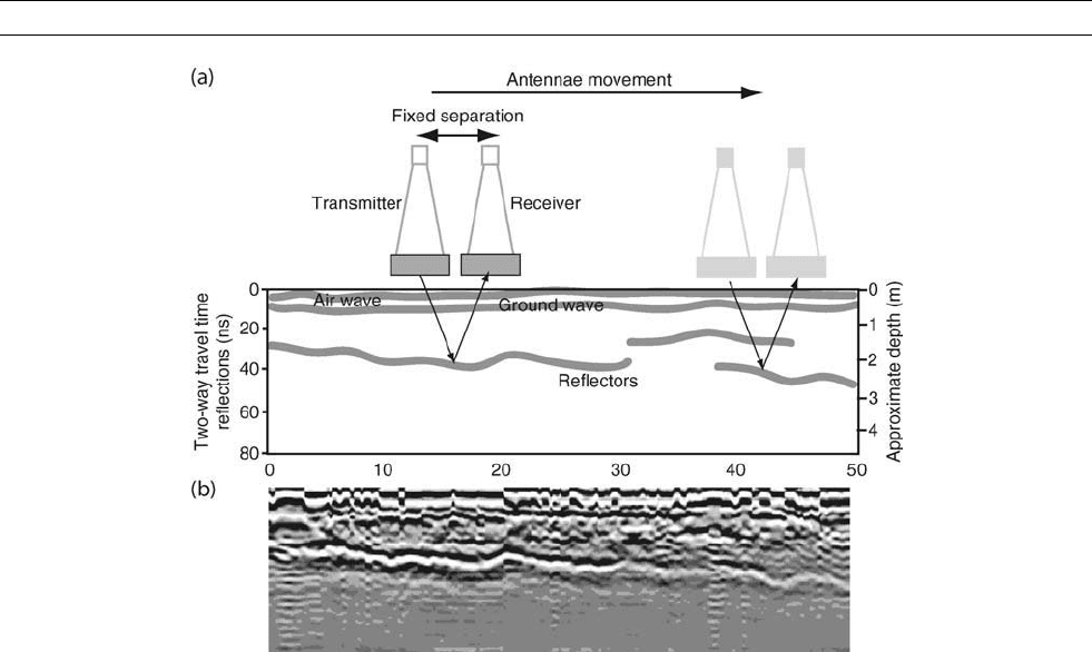
In GPR surveys, pairs of interchangeable radar antennas are used as

a transmitter and receiver, as shown in Figure E13 (Daniels et al.,

1988). A pulse of high-frequency signal is directed into the ground,

and the EM echoes are recorded. Depths of penetration are typically

about 50 m for 10 MHz, 5 m for 100 MHz, and 0.5 m for 1000 MHz.

In environmental studies, the water content dominates the dielectric

properties, as the dielectric permittivity of water is typically ten times

greater than that of solid grains. Thus, GPR is used to map depths to

water tables and soil moisture content. For geotechnical studies,

GPR studies are effective at mapping near-surface engineering struc-

tures, including pipes, cavities, and metal objects.

Summary

There continues to be growth in the use of EM methods for resource

exploration, and for environmental and engineering applications.

These methods are generally rapid and noninvasive, and provide both

a lateral and vertical image of electrical conductivity and dielectric per-

mittivity properties of Earth. The industry has adapted these methods

to operate in a wide range of environments, particularly in the fields

of land, marine, airborne, and downhole studies.

Graham Heinson

Bibliography

Becken, M., and Pedersen, L.B., 2003. Transformation of VLF anomaly

maps in apparent resistivity and phase. Geophysics, 68: 497–505.

Chave, A.D., Constable, S.C., and Edwards, R.N., 1991. Electrical

exploration methods for the seafloor. In Nabighian, M.N. (ed.),

Electromagnetic Methods in Applied Geophysics. Tulsa, OK:

Society of Exploration Geophysicists, pp. 931–966.

Constable, S., Orange, A., Hoversten, G.M., and Morrison, H.F., 1998.

Marine magnetellurics for petroleum exploration. Part 1. A seafloor

instrument system. Geophysics, 63: 816–825.

Daniels, D.J., Gunton, D.J., and Scott, H.F., 1988. Introduction to sub-

surface radar. IEEE Proceedings, 135: 278–320.

Dyck, A.V., 1991. Drill-hole electromagnetic methods. In Nabighian,

M.N. (ed.), Electromagnetic Methods in Applied Geophysics.

Tulsa, OK: Society of Exploration Geophysicists, pp. 881–930.

Edwards, R.N., and Nabighian, M.N., 1991. The magnetometric resis-

tivity method. In Nabighian, M.N. (ed.), Electromagnetic Methods

in Applied Geophysics. Tulsa, OK: Society of Exploration Geophy-

sicists, pp. 47–104.

Edwards, R.N., 1988. A downhole magnetometric resistivity technique

for electrical sounding beneath a conductive surface layer. Geophy-

sics, 53: 528–536.

Edwards, R.N., Lee, H., and Nabighian, M.N., 1978. On the theory

of magnetometric resistivity (MMR) method. Geophysics, 43:

1176–1203.

Friscknecht, F.C., Labson, V.F., Spies, B.R., and Anderson, W.L.,

1991. Profiling methods using small sources. In Nabighian, M.N.

(ed.), Electromagnetic Methods in Applied Geophysics. Tulsa,

OK: Society of Exploration Geophysicists, pp. 105–270.

Hoversten, G.M., Morrison, H.J., and Constable, S., 1998. Marine

magnetellurics for petroleum exploration Part 2. Numerical analy-

sis of subsalt resolution. Geophysics, 63: 826–840.

Figure E13 (a) Schematic of a ground-penetrating radar system to detect subsurface structure. The cross section shows interpreted

reflections from the radargram in the lower figure. The airwave and groundwave are signals that propagate between the transmitter and

receiver through the air and the top few centimeters of the ground, and are therefore almost constant across the profile. (b) Reflections

of high frequency (in this case 200 MHz) EM waves shown as a typical grayscale radargram in the lower figure.

226 EM, INDUSTRIAL USES

McNeill, J.D., 1980. Electromagnetic terrain conductivity measure-

ment at low induction numbers. Technical Note TN-6, Geonics

Limited, Mississauga, Ontario.

McNeill, J.D., and Labson, V., 1991. Geological mapping using VLF

radio fields. In Nabighian, M.N. (ed.), Electromagnetic Methods

in Applied Geophysics. Tulsa, OK: Society of Exploration Geophy-

sicists, pp. 521–640.

McNeill, J.D., 1990. Use of electromagnetic methods for groundwater

studies. In Ward, S.H. (ed.), Geotechnical and Environmental

Geophysics. Tulsa, OK: Society of Exploration Geophysicists,

pp. 191–218.

Nabighian, M.N., and Macnae, J.C., 1991. Time domain electromag-

netic prospecting methods. In Nabighian, M.N. (ed.), Electromag-

netic Methods in Applied Geophysics. Tulsa, OK: Society of

Exploration Geophysicists, pp. 427–520.

Olhoeft, G.R., 1985. Low-frequency electrical properties. Geophysics,

50: 2492–2503.

Palacky, G.J., and West, G.F., 1991. Airborne electromagnetic meth-

ods. In Nabighian, M.N. (ed.), Electromagnetic Methods in Applied

Geophysics. Tulsa, OK: Society of Exploration Geophysicists,

pp. 811– 880.

Vozoff, K., 1991. The magnetotelluric method. In Nabighian, M.N.

(ed.), Electromagnetic Methods in Applied Geophysics. Tulsa,

OK: Society of Exploration Geophysicists, pp. 641–712.

Zonge, K.L., and Hughes L.J., 1991. Controlled source audio-

frequency magnetotellurics. In Nabighian, M.N. (ed.), Electro-

magnetic Methods in Applied Geophysics. Tulsa, OK: Society of

Exploration Geophysicists, pp. 713–810.

Cross-references

EM Modeling, Forward

EM Modeling, Inverse

EM, Industrial Uses

EM, Land Uses

EM, Marine Controlled Source

Magnetometers, Laboratory

Magnetotellurics

Transient EM Induction

EM, LAKE-BOTTOM MEASUREMENTS

Magnetic fields set up by electrical currents flowing in the Earth's

ionosphere and magnetosphere diffuse into the Earth's interior, and

induce electrical currents to flow in the oceans and in conductive

regions in the Earth's interior. Longer period magnetic field variations

have a greater depth of penetration than shorter period variations. By

relating the variations in the electric field to those in the magnetic field

at different locations and over a range of different periods, it is possi-

ble to reconstruct the distribution of electrical conductivity within the

Earth, and from that information, to constrain the temperature, compo-

sition, fluid and volatile content, and state of Earth materials. This

is the magnetotelluric (MT) method (see Magnetotellurics; Galvanic

distortion; EM, land uses).

In order to penetrate deep into the lithosphere and below, long-

period MT measurements are required. Other methods involving only

magnetic field measurements (see Geomagnetic deep sounding; EM,

regional studies) are valid for field variations with periods longer than

2–4 days, and provide information on electrical conductivity of the

mantle at depths below 400 km (Schultz et al ., 1987) (see Mantle,

electrical conductivity, mineralogy). Conversely, the MT method is

usually employed to investigate periods many decades shorter than

this, generally less than 0.2 days. Consequently most MT investiga-

tions are restricted to the crust and uppermost mantle. By extending

the range of MT investigations to longer periods, finer structural

details may be resolved at depth, and information on anisotropy within

the crust and mantle may be returned.

The electric field is measured by monitoring the electrical potential

across (typically) two orthogonal pairs of metal salt electrodes grounded

to Earth and separated by a fixed distance. Electrode noise is a considera-

tion for MT. There is long-period electric field measurement drift due to

variations in electrochemical conditions in the soil, moisture content, and

thermal effects (Perrier and Morat, 2000), and to electrokinetic effects (Tri-

que et al., 2002). To improve the signal-to-noise ratio, a number of deeply

penetrating MT investigations have taken place making use of extremely

long electrode separations, by using leased telephone cables on land

(Egbert et al., 1992), or abandoned submarine telecommunications cables

on the seafloor (see Conductivity, ocean floor measurements).

Schultz and Larsen (1987) proposed that the thermally and electro-

chemically stable environment of lake bottoms might provide an ideal

environment to extend MT into periods of 0.2–4 days and below, thus

spanning the gap in coverage left by conventional MT and magnetic

field methods. While lake-bottom MT shares common features with

ocean bottom MT, the high conductance of marine sediments and the

conductive seawater overburden at most marine study sites shields

the seafloor from the high frequency signals that penetrate to the bot-

tom of lakes, and that can provide higher resolution information on

shallow crustal and upper mantle conductivity structure. While con-

tamination of the EM fields by water motions (such as mesoscale

eddies) impose a low frequency limit to MT in the oceans, this is gen-

erally not a significant consideration in lakes.

A prototype lake-bottom MT station was installed in Lake Washing-

ton, in Seattle, Washington, to form an array of Ag-AgCl electrodes,

with electrode separations of 800–1300 m. This configuration pro-

vided three nonorthogonal components of the electric field, any

two of which could be rotated into orthogonal components. A fluxgate

magnetometer was buried on the adjacent shore, and high-quality MT

data resulted. The MT regional strike direction was seen to be coinci-

dent with the strike delineated by regional seismicity and tectonics.

The effects of a channeled current were seen, attributed to an Eocene

suture zone to the south of the site (Schultz et al., 1987).

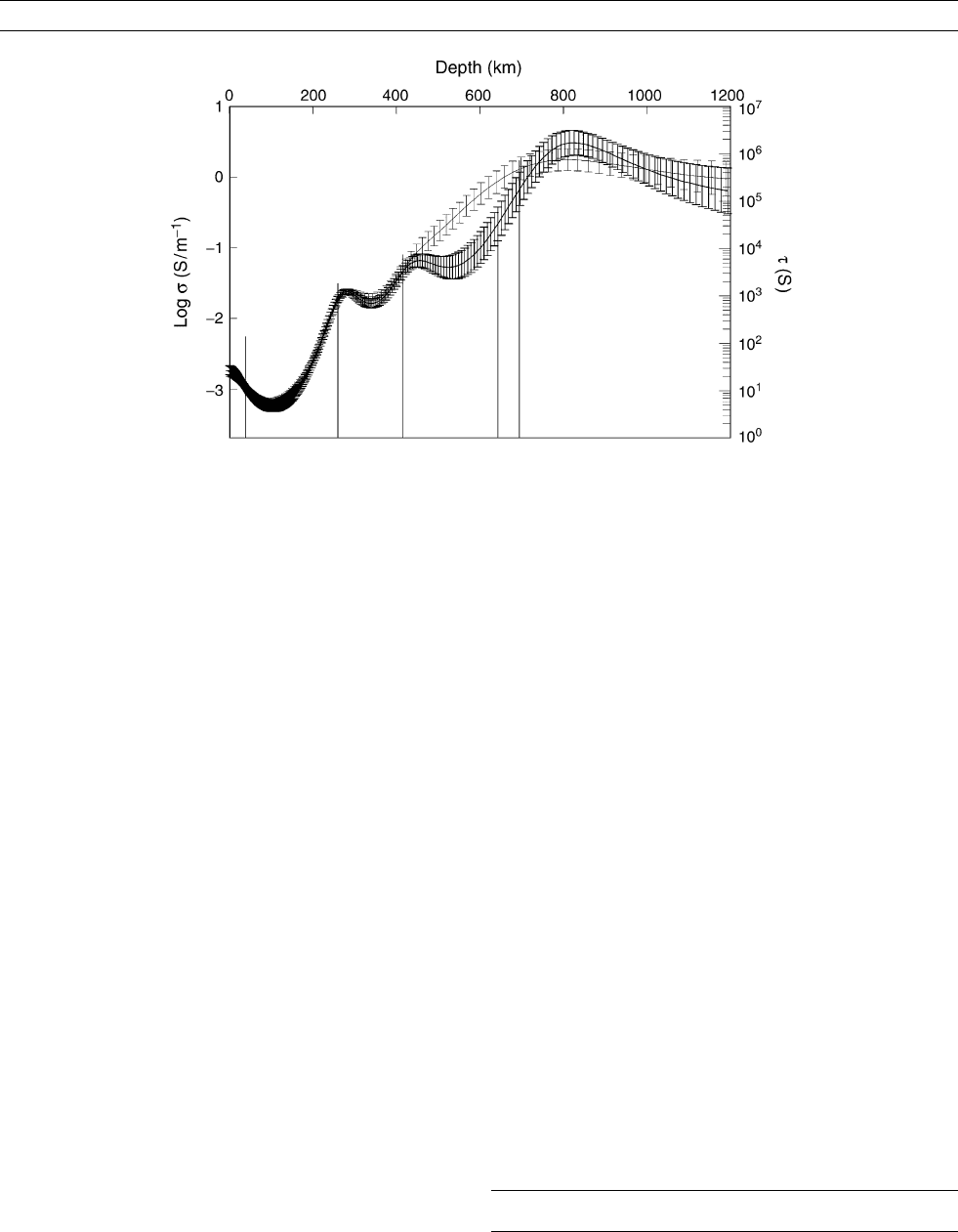
A multiyear lake-bottom MT deployment followed in the Archean

Superior craton of northern Ontario, Canada (Schultz et al., 1987).

More than 2 years of MT data were collected from Carty Lake, follow-

ing the configuration at Lake Washington. Three zones in the mantle

were identified, centered at depths of 280, 456, and 825 km, and

roughly coincident with major seismic discontinuities, where the con-

ductivity increased abruptly (Figure E14). The ability to discriminate

the jump centered at around 456 km was attributed to MT data with

periods of 1 h to 1 week, which were made possible by the stable

lake-bottom installation. No other MT experiment to date has produced

resolving power sufficient to discriminate the 456 km conductivity

increase. The conductance of the upper mantle here was roughly an

order of magnitude higher than that predicted by a standard olivine

model using a standard geotherm. It was determined that either the

upper mantle geotherm was erroneously biased downward, or a dry

olivine upper mantle model was inappropriate.

Jones et al. (2001a,b, 2003) report on the lake-bottom deployment

of compact MT instruments designed for marine use, and of electric

dipole receivers inserted through the ice to the bottom of frozen lakes,

with magnetometers nearby on shore. These installations in roughly

20 lakes were made to probe to the depth of the top of the asthenosphere

beneath the Slave craton in northwestern Canada, in a region of

diamondiferous kimberlite pipes. Their investigations serendipitously

revealed a highly conductive zone at depths of 80 to below 100 km

in the mantle that is interpreted to represent interconnected carbon or

graphite along mineral grain faces. Jones et al. (2003, 2004) determined

that the Superior craton MT data of Schultz et al. (1993) and those of the

Slave craton indicate that while both provinces differ in shallow structure,

on average the deeper mantle sections are nearly identical. Jones et al.

(2003) compared the lake-bottom MT data against earlier data from the

region, and found that these depths had previously been beyond the

EM, LAKE-BOTTOM MEASUREMENTS 227

limits of penetration of conventional MT, but were now resolvable

because of the extended bandwidth available to lake-bottom MT.

Golden et al. (2004a,b) carried out lake-bottom MT measurements

in Woelfersheimer lake near Frankfurt am Main, in 2003. These proto-

type experiments lead to a successful lake-bottom deployment in Ice-

land. While the analysis of these data is ongoing with the aim of

better imaging the putative mantle plume beneath Iceland, a lower

noise level is seen for the Icelandic lake-bottom MT data than for

nearby conventional MT deployments.

Lake-bottom electromagnetic deployments have now been used at

numerous sites in North America, Europe, and Iceland. The experience

indicates that this environment provides a means of extending MT

observations into the mid-mantle, and for improving the ability to

resolve finer structural details than shorter duration, more noise-prone

conventional MT installations.

Adam Schultz

Bibliography

Egbert, G.D., Booker, J.R., and Schultz, A., 1992. Very long period

magnetotellurics at Tucson observatory—estimation of impe-

dances. Journal of Geophysical Research, 97(B11): 15113–15128.

Golden, S., Björnsson, A., Beblo, M., and Junge, A., 2004a. Project

CMICMR: Long-period magnetotellurics on Iceland. American

Geophysical Union, Fall Meeting 2004, abstract #GP11A-0819.

Golden, S., Roßberg, R., and Junge, A., 2004b (im Druck)b. Langper-

iodische MT-Messungen in einem See mit dem Langzeit-Datenlog-

ger Geolore (“Long-periodic MT measurements in a lake with the

long-term datalogger Geolore”), Protocol über das Kolloquium

Elektromagnetische Tiefenforschung, 20.

Jones, A.G., Ferguson, I.J., Chave, A.D., Evans, R.L., and McNeice,

G.W., 2001a. Electric lithosphere of the slave craton. Geology,

29(5): 423–426.

Jones, A.G., Snyder, D., and Spratt, J., 2001b. Magnetotelluric and tel-

eseismic experiments as part of the Walmsley Lake project, north-

west territories: experimental designs and preliminary results,

Current Research 2001-C6, Geological Survey of Canada, 7 pp.

Available at: http://gsc.nrcan.gc.ca/bookstore/

Jones, A.G., Lezaeta, P., Ferguson, I.J., Chave, A.D., Evans, R.L.,

Garcia, X., and Spratt, J., 2003. The electrical structure of the

Slave craton, Lithos, 71: 505–527.

Jones, A.G., and Craven, J.A., 2004. Area selection for diamond

exploration using deep-probing electromagnetic surveying. Lithos,

77: 765–782.

Perrier, F., and Morat, P., 2000. Characterization of electrical daily var-

iations induced by capillary flow in nonsaturated zone. Pure and

Applied Geophysics, 157(5): 785–810.

Schultz, A., Booker, J., and Larsen, J., 1987. Lake bottom magnetotel-

lurics. Journal of Geophysical Research, 92(B10): 10639–10649.

Schultz, A., Kurtz, R.D., Chave, A.D., and Jones, A.G., 1993.

Conductivity discontinuities in the upper mantle beneath a stable

craton. Geophysical Research Letters, 20(24): 2941–2944.

Trique, M., Perrier, F., Froidefond, T., Avouac, J.-P., and Hautot, S.,

2002. Fluid flow near reservoir lakes inferred from the spatial

and temporal analysis of the electric potential. Journal of Geophy-

sical Research, 107(B10): 2239, doi:10.1029/2001JB000482.

Cross-references

Conductivity, Ocean Floor Measurements

EM, Land Uses

EM, Regional Studies

Galvanic Distortion

Geomagnetic Deep Sounding

Magnetotellurics

Mantle, Electrical Conductivity, Mineralogy

EM, LAND USES

Land-based electrical and electromagnetic (E&EM) geophysical meth-

ods have been applied in mapping the electrical conductivity, or the

reciprocal resistivity, structure of the Earth for applications as varied

as general geological mapping; waste site characterization; contamina-

tion delineation; hydrogeological investigations; exploration for

oil and gas, mineral, geothermal, sand, gravel, limestone, and clay;

Figure E14 Electrical conductivity model for lake-bottom MT site, Carty Lake, Superior craton, Canada. The thick curve is the model

of log

conductivity vs depth that has the minimum size of jumps in conductivity (min

log s=dz) of all models that fit the data.

Note the jumps in conductivity centered at 280, 456, and 825 km. The thinner curve is a model with the same properties, but with the

lake-bottom MT data with periods of 2 h to 6 days deleted, showing that the peak at 456 km can only be resolved if the lake-bottom data

are present. The thin vertical bars represent the best-possible fitting model comprised of infinitely thin zones of finite conductance, t.

228 EM, LAND USES

geotechnical investigations of building and road construction sites; loca-

tion and identification of subsurface utilities; unexploded ordnance

detection; and precision agriculture. Geophysical methodologies are

almost as varied as the applications. The electric or magnetic fields or a

combination of both are measured for plane wave or controlled sources

in either the time or the frequency domain. Imaging of subsurface conduc-

tivity structure can extend from simple contouring of the data, to rigorous

and computer-intensive, multidimensional inverse modeling. The depths

of investigation can be a function of operating frequency, decay time,

or the geometric array, ranging from meters to tens of kilometers.

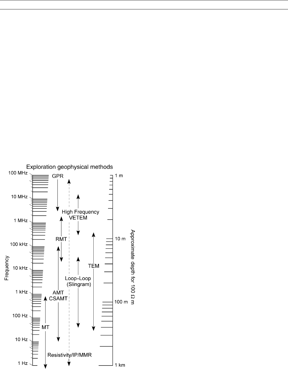
Figure E15 shows a schematic of the frequency range for commonly used

E&EM methods and approximate depths of investigation for an Earth

of 100 O m.

The behavior of E&EM fields is governed by Maxwell's equations

(Ward and Hohmann, 1988). The physical earth parameters determining

the response are the electrical conductivity (s ), or its reciprocal resistiv-

ity (r), the magnetic permeability (m), and the dielectric permittivity (e).

The geophysical EM spectrum ranges from ground-penetrating radar

(GPR) at hundreds of MHz to low frequencies approximating a direct

current (dc) as shown in Figure E15.

Land-based EM systems employ frequencies within the quasistatic

approximation in which displacement currents are ignored, such that

inductive currents predominate and field propagation are diffusive.

GPR systems operate in the high-frequency range where displacement

currents dominate and field propagation is a wave phenomenon. In the

dc limit, the electric field is a potential governed by the Poisson equa-

tion. In most applications it is assumed m = m

(free space), because

magnetic materials are often anthropomorphic artifacts, such as drums

and pipelines. E&EM techniques can directly map the ionic content of

the pore water, an indicator of the subsurface water chemistry and clay

content, which is more difficult to achieve with wavefield methods

such as GPR.

Elect rical resistivi ty

Electrical current at frequencies near the dc limit is injected into the

ground over an array of current electrodes using a transmitter, and

the resulting voltage is measured over a similar array of voltage elec-

trodes. Current can be injected either galvanically or capacitively. The

depth of investigation and resolution are determined by the electrode

array and spacing. A description of the wide variety of electrode arrays

can be found in Telford et al. (1990). Inhomogeneities in the Earth

alter the current flow from what would be present with a uniform

half-space, and are considered as secondary current distributions.

Using modern multielectrode equipment and continuous systems, data

are measured in profile or array configurations so that lateral and ver-

tical resistivity variation can be determined through data inversion.

With a multielectrode galvanic system, 20–100 electrodes are usually

placed equidistantly in an array, which can be both on and below the sur-

face. A computer-controlled switch box connects four electrodes to input

current and measure the resulting voltage. A series of configurations are

measured and stored one after the other, and data are stacked until a certain

noise level is reached or an upper limit on the number of measurements

is attained. Several systems are commercially available and the use of

multielectrode geoelectric measurements has increased dramatically over

the past 5–10 years. Electrical resistance tomography (ERT) is a term

frequently used to describe such systems. Applications are as diverse as

precision agriculture, hydrogeological investigations, waste site character-

ization, road and building foundation investigations, and archaeological

studies. Permanent or semipermanent arrays are often used to monitor

infiltration and containment migration problems.

Continuous systems make measurements continuously as the instru-

ment is towed over the ground. The Danish pulled array continuous

electrical sounding (PACES) system (Srensen, 1996) uses galvanically

coupled steel cylinder electrodes mounted on a tail. The French use

spiked wheels as electrodes or capacitively coupled electrodes mounted

inside plastic wheels (Panissod et al., 1998). In the United States the

OhmMapper system uses a capacitively coupled dipole-dipole array

(Pellerin et al.,2004).

The depth of investigation for electrical resistivity systems is limited by

the power needed to deliver the required current and the wires needed to

support the array. A general estimate for depth of investigation is 40%–

60% of the array geometry. Hence for a transmitter-receiver separation

of 10 m, the expected depth of investigation would be roughly 5 m. For

large depths this entails the use of large amounts of wire, a logistical diffi-

culty. Interpretational complexity increases as different geological struc-

tures are crossed. The electrical resistivity method is most practical in

the 1–50 m depth range.

A question for production surveys of multielectrode systems is

which electrode configurations to use. The choice depends upon opti-

mizing resolution capabilities and the signal-to-noise ratio. Standard

electrode configurations include the Wenner and Schlumberger arrays

where the potential electrodes are inside the current electrodes along

a profile; the dipole-dipole where the current electrodes are offset from

the potential electrodes along a profile; and the pole-dipole and pole-

pole configurations that utilize a distant electrode away from an elec-

trode array. Practically, the Wenner and Schlumberger arrays are most

robust in the presence of cultural noise with a high signal-to-noise ratio,

the dipole-dipole array most rapid for deployment over large areas,

and the pole-pole array fully general in that all arrays are present.

Figure E15 The geophysical EM spectrum showing common

exploration methods and the corresponding frequency range,

or equivalent time, and approximate depth of investigation for

a 100 Om half-space. The dashed line related to the resistivity/

IP/MMR methods indicate the depth of investigation is related

to the array geometry and not the operating frequency.

EM, LAND USES 229

The continuous systems, such as the PACES and OhmMapper, employ

array configurations based on the design of the instrument.

Two-dimensional inversion is the state of the practice for profile-

oriented, electrical resistivity data (Loke and Barker, 1996). Fast

approximate inversion procedures applicable to large data sets are

becoming common along with three-dimensional inversion applicable

to large pole-pole arrays and monitoring systems.

Induced polarization

When electrically polarizable minerals are present in the subsurface,

induced polarization (IP) at the particle interfaces causes the secondary

currents in the vicinity to be out of phase with the applied current

(Fink et al., 1990). Although some IP effects are associated with ionic

double layers on any silicate surfaces, it is clays and sulfides that tend

to exhibit the largest response, thus providing more direct information

on lithology than electrical conductivity alone. Historically the IP

method has been used successfully in delineating porphyry-copper

deposits. More recently IP is used to discriminate between clay-

bearing and clean sand units in groundwater prospecting. As shown

in many case histories and methodology studies, IP is one of the most

powerful techniques for environmental applications. In the 1960s the

use of IP was proposed for landfill characterization and after many

years of GPR, conductivity meters and electrical resistivity surveys,

the use of IP is being shown to be the most accurate tool of the trade.

For accurate IP measurements nonpolarizable electrodes, most often

lead/lead chloride or copper/copper sulfate, are needed resulting in high

survey costs. However, alternative solutions are emerging as smart elec-

trodes, correction schemes for use of ordinary polarizable electrodes,

and measuring strategies allowing for efficient data collection over large

areas are being used.

Magnetometric resistivity

Analogous to the electrical resistivity method, the magnetometric resis-

tivity (MMR) method (Edwards and Nabighian, 1991) is based on the

measurement of low-frequency magnetic fields associated with nonin-

ductive current flow in the ground. Instead of potential electrodes the

magnetic field is measured with coils or magnetometers. Though not

widely utilized, the technique has been successfully used in mineral

exploration, geothermal investigations, and geological mapping related

to environmental applications. Strengths of the method include it being

relatively insensitive to small conductive bodies, and when employing a

vertical electric source, layered structures are not excited and the MMR

response is due solely to three-dimensional targets.

Controlled-source frequency-domain electromagnetics

A number of configurations can be used with controlled-source fre-

quency-domain EM systems (Spies and Frischknecht, 1991). The most

common is the magnetic dipole-dipole or “Slingram” method that

employs a small loop, dipole transmitter and small loop, dipole recei-

ver at multiple-frequencies (Frischknecht et al., 1991). Measurements

can be made of the real component, which is in-phase with the trans-

mitted signal, and the out-of-phase, or quadrature, component. The

ground conductivity meter (GCM) is a subset of the Slingram method

in that it operates where the low frequency inductive approximation is

valid and the quadrature component is linearly proportional to the

apparent ground conductivity. These methods offer the advantage that

ground contact is not necessary, meaning that operation is fast, mini-

mal personnel are required, and continuous data acquisition can be

easily implemented. They have been widely used as profiling instru-

ments with the subsequent interpretation based on the simple apparent

conductivity representation.

Slingram/GCM data have a number of limitations with regard to

quantitative inversion. The secondary field that carries information

about the subsurface conductivity is measured in the presence of

the primary fields, which can be orders of magnitude larger. This

necessitates a compensation of the primary field so that the measured

in-phase component only comes from the secondary field. Accuracy

of the compensation depends heavily on the transmitter-receiver dis-

tance; hence for every transmitter-receiver separation and for every

frequency, the instrument must have a compensation circuit. Instru-

ments with coil separations of less than 60 m and a connecting cable

between the transmitter and receiver are difficult to calibrate and coil

separation errors are detrimental to the accuracy of the in-phase com-

ponent, unless the coil separation is so large and field conditions favor-

able that a good relative accuracy is obtainable. The quadrature

component is relatively insensitive to close separation geometry.

The in-phase component of magnetic dipole-dipole systems is reli-

ably measured with fixed boom systems where the transmitter and

receiver coils are in a rigid frame. For practical reasons these systems

are often small. Small coil separations a few meters above a resistive

ground effectively constitute a nonconductive environment enabling

a primary field zeroing and gain calibration. For coil separations exceed-

ing a few meters it is awkward to get far enough away from the ground.

Consequently, calibration is difficult, impeding a quantitative assess-

ment of the reliability of the data. Calibration can be performed with

calibration coils, but it is still a time-consuming and cumbersome

process.

There is an ongoing debate about the value of having more than one

frequency for geological mapping with small fixed-boom systems. One

side claims that differences in investigation depths are pronounced

enough for multifrequency measurements to be useful. The other side

maintains that for conductivity mapping purposes one frequency is suf-

ficient because the skin depth is large compared with the coil separation

for all appropriate frequencies, meaning that the sensitivity is controlled

by the coil separation. Sounding data can be obtained by using two

dipole orientations (horizontal coplanar and vertical coplanar) and mea-

suring at different heights, however using multiple coil separations

rather than data at different elevations is preferable. The resolution

kernels for soundings at different elevations become almost parallel at

relatively shallow depth thus reducing the independence of the data.

For quadrature data the equivalent half-space is linear in conductiv-

ity and inversion reduces to a simple transformation. However, the

inverse problem is only linear with respect to conductivity at low-

induction number, an assumption that can be poor in many near-

surface environments. An accurate inversion should take into account

the system response: phasing of the instrument, correction for mea-

surement elevation, and calibration factors, as well as the departures

from the low-induction number approximation.

Plane wave electromagnetics

Magnetotellurics is arguably the most developed of all EM methods

because of the elegance of the plane wave source assumption. Used

for deep sounding of the Earth's crust the method has also been used

extensively for oil and gas and geothermal exploration. The complex

impedance of the Earth is inferred from measurements of the natural

electric and magnetic field—or more accurately the voltage measured

across orthogonal electric dipoles and induction coils. The MT source

below 1 Hz is due to currents in the magnetosphere and above that

from worldwide lightning. At about 1 Hz the natural signal strength

is low, but schemes have been developed to compensate. The remote

reference technique makes use of the simultaneous measurements of

the field at multiple sites to removes bias and cultural noise.

The audio magnetotelluric (AMT) and the controlled-source AMT

(CSAMT) methods are applied to hydrological and resource explora-

tion targets (Zonge and Hughes, 1991) with depths of investigation

from tens to hundreds of meters. The AMT method employs natural

signal in the 100 kHz to 10 Hz range; the CSAMT methods uses an

artificial source, traditionally a grounded electrical dipole that domi-

nates the natural field although other systems use a magnetic dipole

source that augments the low-energy signal at frequencies above

1 kHz. With both approaches the source must be far enough away

230 EM, LAND USES

from the receiver array so that the source has lost its dipolar geometry

and is plane wave, but close enough to have an appreciable signal-

to-noise ratio. For a grounded electrical dipole source this distance,

usually measured in skin depth, can be several kilometers and for a

magnetic dipole hundreds of meters.

The RMT method , making use of EM fields from commercial and

military radio transmitters and ambient signals, operates in the fre-

quency range between 10 kHz (VLF transmitters) and 1 MHz (AM

transmitters) (Tezkan, 1999). The VLF transmitting network will be

discontinued in the near future because submarines now are using

satellites for communication, hence there will be a lack of signal in

the lower frequency range severely limiting the use of the method. It

has been used for mapping waste sites and other contaminated areas.

The CSAMT and RMT methods have the significant advantage of

being able to exploit the multidimensional inversion software that

has been well developed in the MT community.

Time-do main electrom agneti cs

With the time-domain, also known as the transient electromagnetic

method (TEM) the Earth is excited by a loop carrying current on the

surface of the Earth. The current is abruptly turned off and currents

within the Earth are induced to maintain continuity of the magnetic

field. The magnetic field decays as the electric currents diffuse through

the ground. Magn etic field measurements can be made in, out or coin-

cident with the transmitter loop. Traditionally, only the vertical compo-

nent is measured, but much information is available in the horizontal

components.

The TEM has gained popularity over the past decade. Being an

inductive method, it is particularly good at mapping the depth and

extent of good conductors, but is relatively poor at distinguishing con-

ductivity contrasts in the low conductivity range. Clay and saltwater

intrusion constitute conductive features of special interest in aquifer

delineation. Hence, the method has been used extensively in hydro-

geophysical investigations.

The very early time EM (VETEM), and equivalent high-frequency

domain systems have been constructed in the nanos econds range

(Wright et al., 2000) for depths of investigation of less than a few

meters. The response in this range spans the region between diffusion

and wave propagation so the data contain information on the conductivity

and permittivity in areas of high conductivity where the GPR signal is

greatly attenuated.

Louise Pellerin

Bibliogr aph y

Edwards, L.E., and Nabighian, M.N., 1991. In Nabighian, M.N. (ed.),

Electromagnetic Methods in Applied Geophysics , Vol. 2, Part A.

Tulsa, OK: Society of Exploration Geophysicists, pp. 47 – 104.

Fink, J.B., McAlister, E.O., Sternberg, B.B., Wiederwilt, W.G., and

Ward, S.H., 1990. Induced polarization . Investigations in Geophy-

sics, Vol 4. Tulsa, OK: Society of Exploration Geophysicists.

Frischknecht, F.C., Labson, V.F., Spies, B.R., and Anderson, W.L.,

1991. Profiling methods using small sources. In Nabighian, M.N.

(ed.), Electromagnetic Methods in Applied Geophysics, Vol. 2,

Part A. Tulsa, OK: Society of Exploration Geophysicists,

pp. 105– 270.

Loke, M.H., and Barker, R.D., 1996. Rapid least-squares inversion

of apparent resistivity pseudosections by a quasi-Newton method.

Geophysical Prospecting , 44: 131– 152.

Panissod, C., Michel, D., Hesse, A., Joivet, A., Tabbagh, J., and

Tabbagh, A., 1998. Recent developments in shallow-depth electri-

cal and electrostatic prospecting using mobile arrays. Geophysics ,

63: 1542 – 1550.

Pellerin, L., Groom, D., and Johnston, J.M., 2003. Characterization of

an old diesel fuel spill? Results of a multireceiver OhmMapper

survey. In Proceedings 73rd Annual Intern ational Meeting . Tulsa,

OK: Society of Exploration Geophysicists, pp. 5008– 5011.

S  rensen, K.I., 1996. Pulled array continu ous electrical profiling. First

Break , 14:85– 90.

Spies, B.R., and Frischknecht, F.C., 1991. Electromagnetic sounding.

In Nabighian, M.N. (ed.), Electromagnetic Methods in Applied

Geophysics, Vol. 2, Part A. Tulsa, OK: Society of Exploration Geo-

physicists, pp. 285–426.

Telford, W.M., Geldart, L.P., and Sheriff, R.E., 1990. Applied Geophy-

sics. Cambridge: Cambridge University Press.

Tezkan, B., 1999. A review of environmental applications of quasi-

stationary electromagnetic techniques. Surveys in Geophysics , 20:

279– 308.

Ward, S.H., and Hohmann, G.W., 1988. Electromagnetic theory for

geophysical applications. In Nabighian, M.N. (ed.), Electromag-

netic Methods in Applied Geophysics, Vol. 1, Tulsa, OK: Society

of Exploration Geophysicists, pp. 313– 364.

Wright, D.L., Smith, D.V., and Abraham, J.D., 2000. A VETEM sur-

vey of a former munitions foundry site at the Denver Federal Cen-

ter. In Proceedings Symposium for the Application of Geophysics

to Environmental and Engineering Problems (SAGEEP) . Denver,

CO. Society of Environmental and Engineering Geophysics,

pp. 459– 468.

Zonge, K.L., and Hughes, L.J., 1991. Controlled source audio-

frequency magnetotellurics. In Nabighian, M.N. (ed.), Electromag-

netic Methods in Applied Geophysics, Vol. 2, Part B. Tulsa, OK:

Society of Exploration Geophysicists, pp. 713– 810.

Cr oss-referenc es

EM Modeling, Inverse

EM, Industrial Uses

EM, Marine Controlled Source

Magnetotellurics

Robust Electromag netic Transfer Functions Estimates

Transient EM Induction

EM, MARINE CONTROLLED SOURCE

Ba ckground

Controlled source electromagnetic (CSEM) mapping of the electrical

conductivity of the seafloor depends on a simple concept of physics.

If a time-varying EM field is generated near the seafloor, then eddy

currents are induced in the seawater and subjacent crust in accordance

with Faraday's law. The outward progress of the currents with time

depends on range and electrical conductivity. In particular, the apparent

speed in the seawater will be slower than that in the less-conductive

crustal zones. Measurements at a remote location of the electric and

magnetic fields associated with the eddy currents may be inverted for

the crustal resistivity structure, if the resistivity and thickness of the

seawater are known.

The concept is easily verified theoretically through an examination of

the governing differential equations. The Maxwell interrelationships

between the electric field E and the magnetic field B in an isotropic,

homogeneous material may be combined as the damped wave equation

r  r  B ¼ ms

þme

; (Eq. 1)

where s, m, and e are the conductivity, permeability, and permittivity of

the material, respectively. A similar equation may be written for the

magnetic field vector B. Equation (1) may be rationalized by

measuring length and time in units of characteristic length L and

characteristic time t ¼ msL

. There results

EM, MARINE CONTROLLED SOURCE 231

rr B ¼

q B

q t

: (Eq. 2)

The second term on the left-hand side of Eq. (2) usually is neglected

in comparison with the first term and the physics simplified to a diffusion

process because the scale L of the experiment is large compared with

ð e= ms

1 =2

or 1= 377s. The omission is equivalent to the neglect of the

magnetic effects of displacement current in comparison with conduction

current. The critical scale is largest for very resistive crystalline rock, hav-

ing a value of the order of few tens of meters. A feel for the time taken for

an EM disturbance to diffuse through a uniform medium may be gained by

evaluating the characteristic time t for a few typical cases. If the scale L is

set to 1 km and the parameter m takes its free space value, then t has value

3.8 s for seawater, typical conductivity 3 S m

 1

, and 1.2, 0.42, 0.12, 0.042

s for crustal resistivities of 1, 3, 10, and 30 O m, respectively. (The charac-

teristic times are approximate and should be treated as upper limits by as

much as a factor of 10 for practical systems.)

CSEM is usually used to explore crustal regions. The rocks that are

often a simple two-phase system consisting of the resistive grain matrix

and conductive pore fluid. Archie's law (Archie, 1942) relates measured

bulk resistivities to porosity estimates. In a general form, it is

¼ a r

 m

; (E q. 3 )

where r

is the measured formation resistivity, r

is the resistivity of

seawater, f is the sediment porosity, a is a constant, and m the cemen-

tation factor. The latter two parameters can be derived from laboratory

measurements and vary between 0 :5 < a < 2 :5 and 1 :5 < m < 3.

Resistivity values for marine sediments near the seafloor where the

porosity is often in excess of 0.5 may be as low as 1 O m.

Practical meth ods: respo nse of a layered earth

A practical CSEM system consists of a transmitter capable of generat-

ing an EM disturbance and one or more receivers which detect the

disturbance at some later time as it passes nearby. In common with

land-based systems used for mineral prospection, the transmitter and

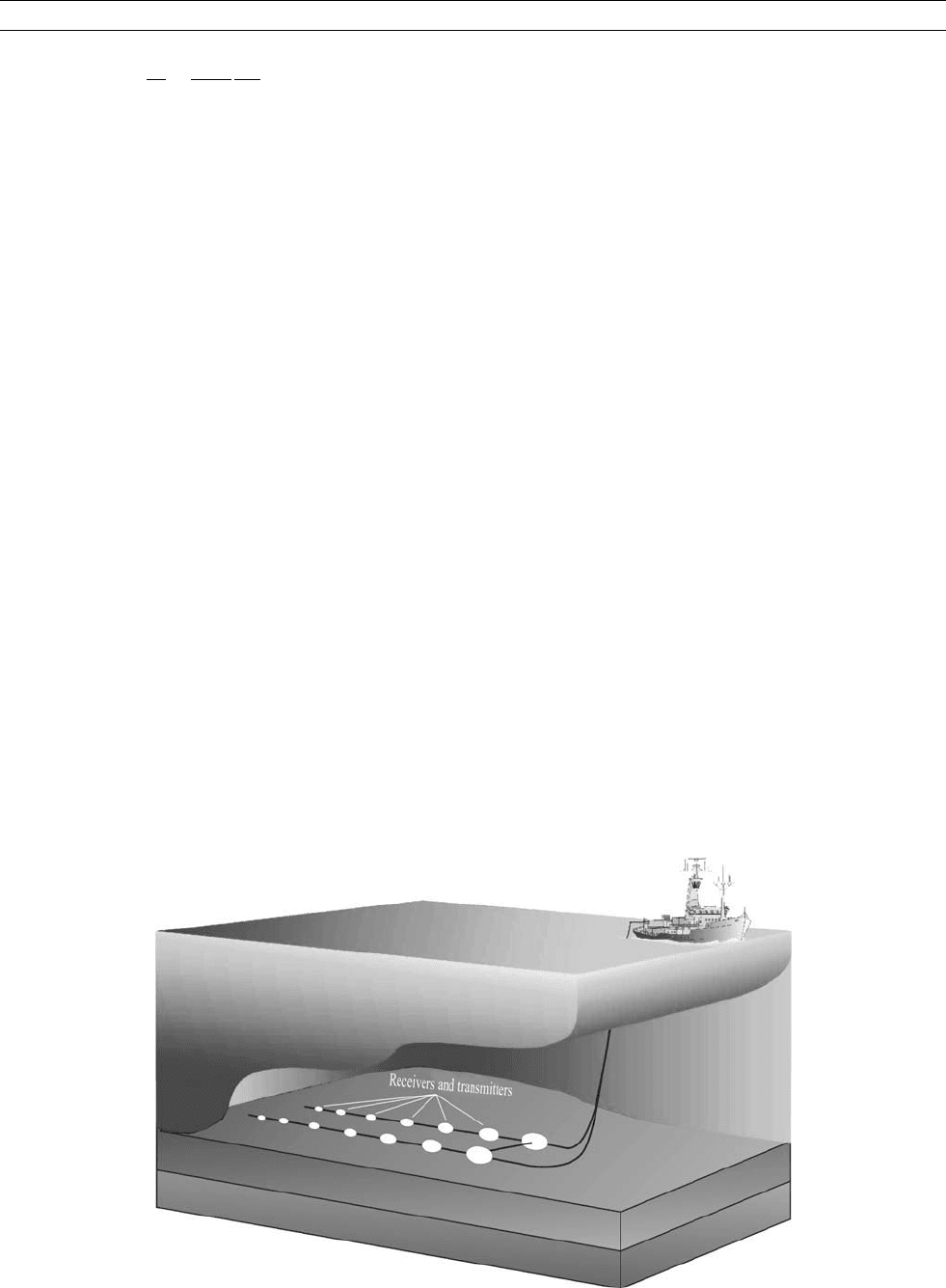
the receiver may be electric and/or magnetic dipoles. Usually, for mar-

ine exploration, both the transmitter and the receivers are near or on

the seafloor, as shown in Figure E16. Further, the system response

can be described in frequency domain or time domain. Both use a con-

tinuous waveform and are essentially equivalent. In particular, delays

in time domain are related to phase changes in frequency domain.

A study of the nature of the response of a layered earth to a time

domain controlled source system is a useful learning exercise, as some

of the physics is counterintuitive. Disturbances from the transmitter

diffuse through the seawater and the seafloor and are seen at the recei-

ver as at least two distinct arrivals separated in time depending on the

conductivity contrast between seawater and subjacent crust. If the

layered seafloor increases in resistivity with depth, then disturbances

propagate laterally more rapidly at depth than immediately beneath

the seafloor. The received signal viewed at different ranges in logarith-

mic time has many of the characteristics of refraction seismic, even

though the process is diffusive, and the signal can be processed using

seismic methods. We use two basic configurations for marine explora-

tion: the horizontal magnetic dipole-dipole and the horizontal electric

dipole-dipole. System geometries can be broadside or in-line. The

two geometries yield different information (Yu and Edwards, 1991;

Yu et al., 1997). For example, the in-line electric dipole-dipole is sen-

sitive to the vertical resistivity whereas its broadside cousin is sensitive

to the horizontal resistivity perpendicular to the line joining the

dipoles. The EM fields impressed in the crust by both the horizontal

magnetic dipole and the horizontal electric dipole have two polariza-

tions. The polarizations are characterized by the absence of a vertical

magnetic field and a vertical electric field, respectively. They average

the resistivity in two different ways. If these averages are different,

then the medium appears to be only laterally isotropic. Data collected

over layered Earth structures must be interpreted using software

including anisotropy either as multiple fine isotropic layers or, better,

as a few anisotropic layers.

By way of example, a summary of the layered earth responses for

the electric dipole-dipole system for the in-line configuration, follow-

ing Chave and Cox (1982), Edwards and Chave (1986), and Cheesman

et al. (1987) is presented here. The seawater has a finite thickness

and an electrical conductivity s

. The permittivity of the air is e.

The subjacent crust has N layers with thicknesses d

; d

; ...; d

N1

and conductivities s

; s

; ...; s

, respectively. A current I is switched

on at time t ¼ 0 and held constant in a transmitting electric dipole of

Figure E16 A towed electric seafloor array. Transmitter and receiver electrodes are interchangeable and pairs can be connected to

generate many dipole-dipole configurations.

232 EM, MARINE CONTROLLED SOURCE

length Dl. The expression for the Laplace transform of the step-on

transient electric field at the seafloor for the in-line electric dipole-

dipole geometry, dipole separation L, is given in terms of s, the Laplace

variable. It is

IDl

2ps

FðsÞþGðsÞ½; (Eq. 4)

where F and G are the Hankel transforms

FðsÞ¼

þ Y

l J

ðlLÞdl; (Eq. 5)

GðsÞ¼ðs=LÞ

þ Q

ðlLÞdl; (Eq. 6)

and the included Laplace transform of the source dipole moment is IDl=s.

If the magnetic effects of displacement currents in the earth are

neglected, then the parameters Y

and Q

are given for the sea layer as

þ sey

tan hðy

sey

þ s

tan hðy



(Eq. 7)

and

þ u

tan hðy

þ y

tan hðy



; (Eq. 8)

where the EM wavenumbers in the ground and in the air are given by

¼ l

þ sms

and u

¼ l

þ s

me.

The parameters Q

and Y

are evaluated through the downcounting

recursion relationships

iþ1

þ y

tan hðy

þ s

iþ1

tan hðy



; (Eq. 9)

and

iþ1

þ m

tan hðy

þ y

iþ1

tan hðy



; (Eq. 10)

where the starting values are Y

¼ y

and Q

¼ m

respectively. The wavenumbers y

are defined by y

¼ l

þ sms

The Y and Q functions denote the polarizations characterized by the

absence of a vertical magnetic field and a vertical electric field, respec-

tively. The Y function yields the DC “resistivity” response at late time

(Edwards, 1997).

The corresponding form for the broadside electric dipole-dipole

geometry is as given in expression (4) but with alternative definitions

for F and G.

The methods for inverting the Hankel and Laplace transforms are

fully described in the theoretical papers listed above. All other geome-

tries are a linear combination of the in-line and broadside responses.

The frequency domain response of the dipole may be obtained by

multiplying the step-on response by s to get the impulse response

and then replacing s by io where o is the angular frequency of the

harmonic current. The inverse Hankel transform becomes a complex

function having a phase and an amplitude.

The theory may be extended to include the effects of anisotropy

caused by interbedding. The coefficient of anisotropy k is defined

by k ¼

ﬃﬃﬃﬃﬃﬃﬃﬃﬃﬃﬃﬃ

, where s

and s

are the tangential and normal

conductivities in any given layer. The coefficient cannot be smaller

than unity. We modify the form of y only in expression (9) to

¼ k

þ sms. In both expressions (9) and (10), s is replaced by

whereever it occurs.

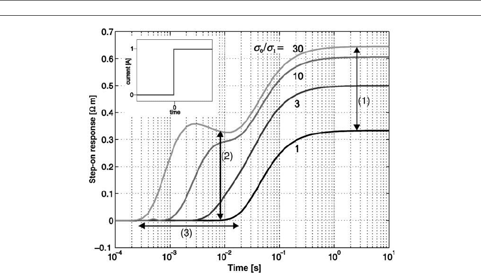
Response curves

The step-on response of a double half-space to the in-line electric

dipole-dipole system is shown in Figure E17. The seawater is

assigned a conductivity of 3 Sm

1

while the subjacent crust has con-

ductivities of 3, 1, 0.1, and 0.3 Sm

1

, respectively. The vertical axis

has been scaled to yield the DC apparent resistivity at late time. The

horizontal axis is in logarithmic time for a transmitter-receiver separa-

tion L of 260 m. (Absolute time may be estimated for any system,

given a conductivity s and a value for L,asm

=c, where c is a con-

stant with a value of about 5. Progress of disturbances through several

zones of differing conductivity may be obtained by summing such

estimators.)

The curves have three characteristics from which the conductivity of

the crust may be obtained. There is late-time variation in amplitude

(Label 1), which is less sensitive with increasing conductivity contrast.

There is an early time change in amplitude which depends on the sea-

floor conductivity (Label 2). The location in time of this initial change

is a strong function of seafloor conductivity (Label 3). A robust esti-

mate of determining apparent resistivity from time-domain curves

may be obtained from the maximum in the early time gradient of the

response curve. The same information may be gleaned from amplitude

and phase curves in the frequency domain.

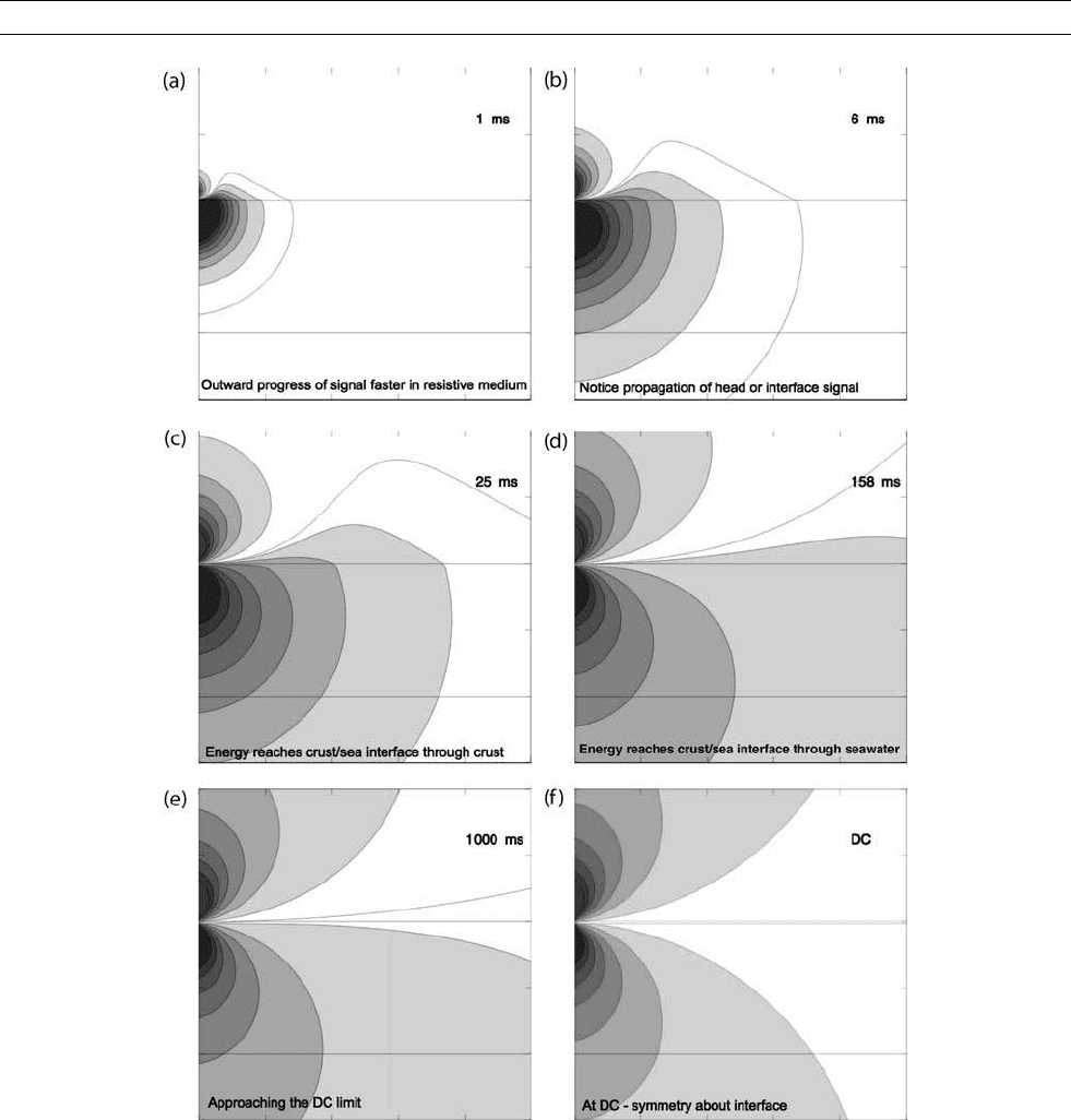
Electromagnetic refraction

Cross sections of the diffusion of current from a 2D electric dipole at

the junction of two half-spaces representing seawater and the subjacent

crust may be used to illustrate the origin of the two arrivals. The diffu-

sive process is plotted as a series of contour maps for increasing time

steps, as shown in Figure E18a through E18f. The magnetic field is out

of the slide, the electric field is in the plane. The model is 500 m

and

the seawater and crust have conductivities of 3 and 0.5 Sm

1

. The

contours, originally shown by Edwards (1988), are current streamlines

and the shading is proportional to the size of the electric field.

The process can be considered as a form of EM refraction, even

though it is diffusive, because of the similarity of the lateral movement

of the current flow pattern and the seismic head wave. Consider the

direction of the Poynting vector

P 

E 

B. Clearly, the first arrival

at a receiver dipole is a disturbance that has propagated through the

more resistive zone, the crust. In the progress of the diffusion, energy

migrates upward from the lower medium through the seafloor. At later

times the signal that propagates through the seawater arrives and at the

static limit (DC) symmetry is reached about the surface. The maps are

consistent with the type curves presented earlier.

Seismic style displays

An impulse response may be obtained as the derivative with respect to

logarithmic time of the step-on response. In the displays that follow,

the normalized impulse response is plotted as a function of logarithmic

time and logarithmic transmitter-receiver separation. The amplitude

scaling, which varies from figure to figure, yields the same curve at

every offset for a simple double half-space. The curve just moves to

later time as the separation increases. The in-line electric dipole-dipole

response has two peaks in the double half-space impulse response cor-

responding to energy that has propagated through the sea and the crust,

respectively. The crustal peak is always at earlier time. Its broadside

cousin also has two features but of different sign. The crustal peak is

positive whereas the seawater trough at later time is negative.

The air wave

Of particular concern to companies that explore in shallow waters such as the

shelf seas is the so-called air wave. Some portion of the EM energy travels

upward to the sea surface, through the air to the vicinity of the receiver and

then downward to the receiver on the seafloor. The up-over-down path can

in some instances be faster than any direct path through the seawater or the

EM, MARINE CONTROLLED SOURCE 233

subjacent crust. Compare the two models shown in Figure E19a and E19b

and the stacked impulse response of these models shown in Figure E19c

through E19f, for the in-line and broadside geometries. The sea layer in

the first model is infinitely thick while that in the second has a finite thick-

ness of 200 m. As the transmitter-receiver separation increases, the air

wave which initially appears at later time appears to move to relatively ear-

lier times and at large separations contaminates the disturbance traveling

through the crust. From a practical point of view, the air wave signature

is easily removed in the inversion of data provided sufficient dynamic

range in the receiver electronics is available to record it properly.

The resistive zone at depth

In the second example, the responses of a double half-space model

modified by the inclusion of a rapid increase in resistivity at a depth

of 200 m have been computed. They are shown in Figure E20b

and compared with the base response of the half-space model, Figure

E20a. The stacked impulse responses for the in-line and broadside

geometries are shown in Figure E20c through E20f. Notice the distinct

refraction visible in the early time crustal response when the EM

disturbance sees the resistive buried zone. The location of the refraction

in space and its slope on the log time vs log separation diagram may be

used to infer the depth to and conductivity of the resistive zone.

Case histories

Gas hydrates in Cascadia

A report of an EM survey for gas hydrate off the west coast of Vancou-

ver Island, Canada, is presented by Schwalenberg et al. (2005) using

apparatus originally developed by Yuan and Edwards (2000). Natural

gas hydrates are ice-like solids found in seafloor sediments. They con-

sist of gas molecules, mainly methane, contained in a cage-like clath-

rate structure of water molecules. They form under low-temperature

and high-pressure conditions, typically in the uppermost few hundreds

of meters of sediments in water depth exceeding about 500 m. The

global abundance of methane frozen in hydrate exceeds the amount

of all other known fossil hydrocarbon resources. Hydrate clearly has

a huge potential as a future energy resource. A gas hydrate deposit

can be generally identified in a seismic section by the occurrence of

a bottom-simulating reflector (BSR) which is associated with the base

of the hydrate stability field. The base is a transition zone between

hydrate-bearing sediments above it and free gas and water below it.

The location of the zone is temperature controlled and depends on

the ambient geothermal gradient. The target area is located on the

accretionary prism of the Cascadia margin in close vicinity of ODP

Site 889, as shown in Figure E21. Here, several seismic blank zones

were observed over a vent field which covers an area of roughly

1km 3 km. The largest, blank zone 1 is called the Bullseye vent

and has a seafloor diameter of about 400 m.

The CSEM experiment was conducted in SW-NE direction, into the

prevailing wind and current, along a profile intersecting the Bullseye

and approaching the other vent sites, making measurements at 28 sites

with a spacing between sites of 250 m. The seafloor array is towed in

direct contact with the soft marine sediments, as sketched in

Figure E22. At the forward end, a heavy weight (pig) is attached

to keep the system in contact with the seafloor. It is followed by a

transmitter dipole (TX) 124 m long and, in this experiment, just two

receiver dipoles (RX1) and (RX2), each 15 m long located at distances

and r

of 174 and 292 m from the transmitter cable, respectively.

While the system is operated in the time domain, using a square cur-

rent waveform with a peak-to-peak amplitude of 20 A and a period

Figure E17 Normalized step-on responses calculated on the interface between two half-spaces to the in-line electric dipole-dipole

system. The conductivity of the upper half-space is 3 S m

1

, for the lower half-space conductivities of 0.3, 0.1, 1, and 3 S m

1

have

been assigned. The separation between transmitter and receiver is 260 m. For a conductivity contrast between seawater and

subjacent crust larger than 10 the arrival through the signal through the seawater at later times can be clearly separated from the earlier

arrival through the crust. In addition, three different effects are noticeable: (1) Amplitude variations at late times depend on the

conductivity contrast, but are mainly due to current flow through the seawater; (2) amplitude variations at earlier times depend on

the seafloor conductivity; (3) the location in time to the initial change is a function of the seafloor conductivity (after Edwards and

Chave, 1986).

234 EM, MARINE CONTROLLED SOURCE

of 6.6 s, the data analysis and inversion to a multilayered model is

completed in frequency domain using phase data only in the band

from 0.5 to 100 Hz.

Simplified results for a half-space model are plotted in Figure E23a

for both receiver separations over a compatible seismic section,

Figure E23b. Two pronounced resistivity anomalies are visible along

the profile which are in striking agreement with the seafloor projec-

tions of the vent sites from the seismic section. The resistivity values

within the anomalous zones are higher for the larger separation

RX2 than those for RX1 and rise up locally to more than 5 m over

the regional background, which lies between 1:1 and 1:5 O m. The

gas hydrate concentrations derived from the resistivity profile, shown

in Figure E24, over the vent sites exceeds 50% at maximum and about

25% on average of the available pore space.

The resolution of the CSEM method does not permit a detailed ana-

lysis of the distribution of the resistive elements within the blank zones

but it does provide an integrated value. Assuming that the increase in

resistivity is due to a higher hydrate concentration, the latter may be

converted to total mass of hydrate and then to total available methane.

A rough estimate can be made for the Bullseye vent assuming a

cylindrical volume, with diameter and depth of 400 and 200 m, respec-

tively. Twenty five percent of the available pore space corresponds to

3.8 million m

. With a solid to gas ratio of hydrate of 1:164, the related

methane gas volume at STP is 0.62 billion (US) cubic meters.

Figure E18 Diffusion in a double half-space. (a–f) Contour maps showing the diffusion proceeding with time of a current from a

2D electric dipole at the interface of two half-spaces representing seawater (3 Sm

1

) and subjacent crust (0.5 Sm

1

). The model is

500 m

. Contours are current streamlines of the electric field and the shading is proportional to the size of the field (after Edwards,

2006).

EM, MARINE CONTROLLED SOURCE 235