Greenwood D.T. Advanced Dynamics
Подождите немного. Документ загружается.


6
Introduction to numerical methods
Digital computers are used extensively in the analysis of dynamical systems. The equations
describing the motion of a system are partly dynamic and partly kinematic in nature. In either
case, they take the form of ordinary differential equations which are nonlinear, in general.
These differential equations are usually written with time as the independent variable, and
time is assumed to vary in a continuous manner from some initial value, frequently zero, to
a final value.
In any representation using digital computers, the time can assume only a finite number of
discrete values. The differential equations of the system are replaced by difference equations.
The solutions of these difference equations are not the same, in general, as the solutions
of the corresponding differential equations at the given discrete times, thereby introducing
computational errors. More importantly, if parameters such as step size are not properly
chosen, a given numerical procedure may produce an apparent unstable response for a
system that is actually stable.
In this chapter, we shall begin with a brief discussion of the interpolation and extrapolation
of digital data. Then we will proceed with a discussion of various algorithms for the numer-
ical integration of ordinary differential equations. The errors arising from these numerical
procedures will be discussed, and questions of numerical stability will be considered.
Another important consideration in the numerical analysis of dynamical systems lies in
the proper representation of geometrical constraints. Even if the physical system is stable,
there may be numerical instabilities resulting from the method of applying constraints. We
shall discuss methods of representing constraints and will analyze their stability.
Finally, a topic of great interest is that of error detection and correction. One approach
is to use integrals of the motion, that is, functions whose values remain constant during the
motion. Examples are the energy or angular momentum functions associated with certain
systems. Any deviations from the expected values of these functions serve as indicators of
errors and are the starting point for possible corrections. These possibilities will be discussed.
6.1 Interpolation
Polynomial approximations
Consider a function of time f (t) whose values are given at the (n + 1) distinct points
t
0
, t
1
,...,t
n
. It is always possible to find an interpolating polynomial of degree n which

330 Introduction to numerical methods
passes exactly through these (n + 1) points. Let us choose
P
n
(t) = a
0
+ a
1
t +···+a
n
t
n
(6.1)
as the approximating polynomial to y = f (t) and let
y
i
= f (t
i
) (6.2)
We can determine the (n + 1) coefficients a
o
, a
1
,...,a
n
from the (n + 1) equations
y
i
=
n
k=0
a
k
t
k
i
(i = 0, 1,...,n) (6.3)
which are linear in the as. For distinct times t
0
, t
1
,...,t
n
, a solution for the asisalways
possible because the determinant of their coefficients is always nonzero. Thus, we can obtain
the interpolating polynomial P
n
(t).
Lagrange’s interpolation formula
An alternative form of the same interpolating polynomial can be obtained by first using the
notation
i
(t) = (t − t
0
)(t −t
1
) ···(t −t
i−1
)(t −t
i+1
) ···(t −t
n
) (6.4)
We note that the factor (t − t
i
) is omitted. Now define a sampling polynomial
δ
i
(t) =
i
(t)
i
(t
i
)
(i = 0, 1,...,n) (6.5)
which is a polynomial of degree n in t. It has the property that it is equal to zero at all
the sampling times t
0
, t
1
,... except at t
i
where its value is one. It is apparent, then, that a
polynomial of degree n which passes through the (n + 1) discrete points is
P
n
(t) =
n
i=0
y
i
δ
i
(t) =
n
i=0
y
i
i
(t)
i
(t
i
)
(6.6)
This is the Lagrange interpolation formula.
An estimate of the error in P
n
(t) can be expressed as a polynomial of degree (n + 1) in t.
Moreover, we know that the error is zero at the (n + 1) points t
0
, t
1
,...,t
n
. So let us assume
that
y(t) ≈ P
n
(t) + C(t −t
0
)(t −t
1
) ···(t −t
n
) (6.7)
where C is a constant to be determined. Now let us differentiate this equation (n + 1) times
with respect to t. The terms arising from P
n
(t) will disappear completely, and we need to
consider only the term Ct
n+1
since the others will vanish upon differentiation. With the aid
of the mean value theorem, we can write
y
(n+1)
(ξ) = (n + 1)!C (t
0
<ξ<t
n
) (6.8)

331 Interpolation
where y
(n+1)
is the (n + 1)th time derivative of y(t). Thus, from (6.7) and (6.8), we obtain
y(t) = P
n
(t) +
(t −t
0
)(t −t
1
) ···(t −t
n
)
(n + 1)!
y
(n+1)
(ξ) (6.9)
The second term on the right represents the error R
n
(t), that is,
R
n
(t) =
(t −t
0
)(t −t
1
) ···(t −t
n
)
(n + 1)!
y
(n+1)
(ξ) (6.10)
It should be noted that the error in the polynomial approximation does not necessarily
decrease with increasing n. This is particularly true when the sample times t
0
,...,t
n
are
equally spaced and the evaluation occurs at a time t near the limits of the overall interval
[t
0
, t
n
]. The problem arises for functions such as tan t,lnt, and 1/(1 +t)
2
whose Taylor
series each have a finite radius of convergence. Although there is an exact match of P
n
(t)
and y(t)atthe(n + 1) discrete points, there is no restriction on the derivatives at these
points. Thus, for polynomials of relatively high degree, it is possible for large errors to
occur between sample times. This is known as the Runge phenomenon. On the other hand,
functions such as sin t and e
t
, whose Taylor series representations have no convergence
problems, will not be subject to these large errors.
Divided difference
Consider the polynomial P
n
(t) passing through the (n + 1) points (y
i
, t
i
) where i =
0, 1,...,n. Define the divided difference
[t
a
, t
b
] = [t
b
, t
a
] =
y
b
− y
a
t
b
− t
a
(6.11)
Similarly, a second-order divided difference is
[t
a
, t
b
, t
c
] =
[t
b
, t
c
] −[t
a
, t
b
]
t
c
− t
a
(6.12)
Again, the order of the arguments makes no difference. More generally, for the (n + 1)
times t
0
,...,t
n
,thenth-order divided difference, written in terms of (n − 1)th-order divided
differences, is
[t
0
, t
1
,...,t
n
] =
[t
1
, t
2
,...,t
n
] −[t
0
, t
1
,...,t
n−1
]
t
n
− t
0
(6.13)
Divided differences can be used in expressing the interpolating polynomial P
n
(t). Con-
sider Newton’s interpolation formula:
P
n
(t) = y
0
+ (t − t
0
){[t
0
, t
1
] +(t −t
1
)[ [t
0
, t
1
, t
2
] + (t − t
2
)([t
0
, t
1
, t
2
, t
3
] +···)]} (6.14)
where the expression is continued until [t
0
, t
1
,...,t
n
] appears.
The coefficients to be used in Newton’s interpolation formula can be computed with
the aid of a divided difference table. For example, consider the case of four sample times

332 Introduction to numerical methods
t
0
, t
1
, t
2
, and t
3
. The corresponding divided difference table is
t
0
t
1
t
2
t
3
y
0
y
1
y
2
y
3
[t
0
, t
1
]
[t
1
, t
2
]
[t
2
, t
3
]
[t
0
, t
1
, t
2
]
[t
1
, t
2
, t
3
]
[t
0
, t
1
, t
2
, t
3
]
As a numerical example, consider the function y = log
10
t and assume unit time intervals.
t log
10
t [·, ·][·, ·, ·][·, ·, ·, ·]
1
2
3
4
0.00000
0.30103
0.47712
0.60206
0.30103
0.17609
0.12494
−0.06247
−0.02558
0.01230
The cubic curve passing through the four given points is found by using Newton’s interpo-
lation formula with the numerical coefficients obtained from the first entry of each column.
Thus, we obtain
P
3
(t) = 0 + (t − 1){0.30103 + (t − 2)[−0.06247 +(t −3)(0.01230)]}
For the case t = 2.5, for example, the interpolation result is
P
3
(2.5) = 1.5{0.30103 + 0.5[−0.06247 − 0.5(0.01230)]}=0.40008
The actual value is log
10
2.5 = 0.39794.
An alternate form of Newton’s interpolation formula is
P
n
(t) = y
0
+ (t − t
0
)[t
0
, t
1
] +(t −t
0
)(t −t
1
)[t
0
, t
1
, t
2
]
+···+(t − t
0
) ···(t −t
n−1
)[t
0
,...,t
n
] (6.15)
This leads to an error or remainder term of the form
R
n
(t) = (t − t
0
) ···(t −t
n
)[t
0
, t
1
,...,t
n
, t] (6.16)
which is obtained by considering t to be an additional data point and writing the next
term, recalling that there would be zero error at time t if the additional term R
n
(t)is
included. Comparing this result with (6.10), and assuming that t is an interior point, we find
that
[t
0
, t
1
,...,t
n
, t] =
y
(n+1)
(ξ)
(n + 1)!
(t
0
<ξ<t
n
) (6.17)

333 Interpolation
Now eliminate t and obtain
[t
0
,...,t
n
] =
y
(n)
(ξ)
n!
(t
0
<ξ<t
n
) (6.18)
For the case n = 0, (6.17) reduces to
[t
0
, t] =
y(t) − y
0
t −t
0
=
˙
y(ξ )(t
0
<ξ<t) (6.19)
which is the mean value theorem.
Forward and backward differences
Let us consider differences associated with a uniform time interval t = h. The forward
difference operator which operates on a function of time f (t )isgivenby
f (t) = f (t + h) − f (t) (6.20)
or
f
n
= f
n+1
− f
n
(6.21)
The forward difference operator has the property of linearity, that is,
[af(t) + bg(t)] = a f + bg (6.22)
where a and b are constants. Furthermore, for a product of two functions of time,
[ f (t )g(t)] = f (t + h)g(t + h) − f (t)g(t ) (6.23)
or
( f
n
g
n
) = f
n+1
g
n+1
− f
n
g
n
= f
n+1
g
n+1
− f
n+1
g
n
+ f
n+1
g
n
− f
n
g
n
= f
n+1
g
n
+ g
n
f
n
= g
n+1
f
n
+ f
n
g
n
(6.24)
where the last equality is obtained by symmetry. For a quotient, we have
f
n
g
n
=
g
n
f
n
− f
n
g
n
g
n
g
n+1
(6.25)
The second forward difference is
2
f
n
= ( f
n
) = ( f
n+2
− f
n+1
) −( f
n+1
− f
n
)
= f
n+2
− 2 f
n+1
+ f
n
(6.26)
In a similar manner, we find that
3
f
n
= (
2
f
n
) = f
n+3
− 3 f
n+2
+ 3 f
n+1
− f
n
(6.27)
4
f
n
= f
n+4
− 4 f
n+3
+ 6 f
n+2
− 4 f
n+1
+ f
n
(6.28)
and so on.

334 Introduction to numerical methods
If f (t) is a polynomial in t, then each forward difference operation reduces its degree by
one. For example, suppose that
f (t) = a
N
t
N
+ a
N −1
t
N −1
+···+a
0
(6.29)
Then
f = a
N
[(t + h)
N
− t
N
] +···
= a
N
Nht
N −1
+··· (6.30)
2
f = a
N
N (N − 1)h
2
t
N −2
+··· (6.31)
k
f = a
N
N (N − 1) ···(N − k + 1)h
k
t
N −k
+··· (6.32)
Hence, we find that
N
f = a
N
N !h
N
(6.33)
and
N +1
f = 0 (6.34)
Forward differences are related to the corresponding derivatives with respect to time at
the middle of the sampling range in t. For example,
f
n
h
=
f
n+1
− f
n
h
≈
˙
y
n+
1
2
(6.35)
2
f
n
h
2
=
f
n+2
− 2 f
n+1
+ f
n
h
2
≈
¨
y
n+1
(6.36)
which can be regarded as central difference approximations to the time derivatives at the
given points. More generally, we find that
k
f
n
h
k
≈
d
k
f
dt
k
t
n
+
1
2
kh
(6.37)
and in addition,
k
f
n
h
k
= f
(k)
(ξ)(t
n
<ξ<t
n
+ kh) (6.38)
As an example, suppose that
f (t) = a
3
t
3
+ a
2
t
2
+ a
1
t +a
0
(6.39)
Then,
f (t) = f (t + h) − f (t)
= a
3
(3ht
2
+ 3h
2
t + h
3
) +a
2
(2ht + h
2
) +a
1
h (6.40)
On the other hand,
˙
f (t) = 3a
3
t
2
+ 2a
2
t +a
1
(6.41)

335 Numerical integration
and
h
˙
f
t +
1
2
h
= 3a
3
h
t
2
+ ht +
1
4
h
2
+ 2a
2
h
t +
1
2
h
+ a
1
h (6.42)
Upon comparing the right-hand sides of (6.40) and (6.42), we see that they differ only in
terms of order h
3
.
From (6.21) and (6.26), we find that forward differences involve present and future data,
but one may also define a difference operator which uses present and past data. This is the
backward difference operator ∇. Its defining equation is
∇ f (t) = f (t) − f (t −h) (6.43)
or
∇ f
n
= f
n
− f
n−1
(6.44)
In addition, we find that
∇
2
f
n
= f
n
− 2 f
n−1
+ f
n−2
(6.45)
∇
3
f
n
= f
n
− 3 f
n−1
+ 3 f
n−2
− f
n−3
(6.46)
∇
4
f
n
= f
n
− 4 f
n−1
+ 6 f
n−2
− 4 f
n−3
+ f
n−4
(6.47)
and
∇
k
f
n
h
k
≈
d
k
f
dt
k
t
n
−
1
2
kh
(6.48)
In applying the interpolating polynomial P
n
(t) we have assumed that the time t liesinthe
interval [t
0
, t
n
]. On the other hand, we can use the same polynomial P
n
(t) in the process of
extrapolation to estimate values of f (t) for times outside the given interval. If t is slightly
greater than t
n
, for example, then (6.17) becomes
[t
0
, t
1
,...,t
n
, t] =
y
(n+1)
(ξ)
(n + 1)!
(t
0
<ξ<t) (6.49)
More explicitly, if we assume a uniform time interval h, and set t = t
n+1
, then we find from
(6.16), that the error is equal to the remainder term
R
n+1
= (t
n+1
− t
0
) ···(t
n+1
− t
n
)
y
(n+1)
(ξ)
(n + 1)!
= h
n+1
y
(n+1)
(ξ)(t
0
<ξ<t
n+1
) (6.50)
This is the error in extrapolating to the (n + 1)th step, using the data of the previous n steps,
including the initial value y
0
.
6.2 Numerical integration
In the study of dynamical systems we consider, in general, ordinary differential equa-
tions with time as the independent variable. If one uses Lagrangian methods, the resulting

336 Introduction to numerical methods
second-order equations of motion are nonlinear, in general, but are always linear in the
¨
qs.
Usually each second-order differential equation is converted to two first-order equations
before numerical integration takes place, resulting in the solution for the dependent vari-
ables as functions of time. Numerical integration is accomplished by first converting the
differential equations to difference equations. These equations are then solved at discrete
instants of time. The solutions of the difference equations ideally should be the same as
the solutions of the differential equations evaluated at the discrete times. Now let us con-
sider some of the numerical procedures or algorithms used in the integration of ordinary
differential equations. The errors associated with these methods will be evaluated.
Euler’s method
Let us begin with a single first-order differential equation
˙
y = f (y, t) (6.51)
Choose a step size t = h and assume that the initial condition y(t
0
) = y
0
is given. The nu-
merical solution for y(t)att = t
1
, t
2
, t
3
,...is obtained by repeating the following sequence
of calculations:
(1)
˙
y
n
= f (y
n
, t
n
) (6.52)
(2) y
n+1
= y
n
+ h
˙
y
n
(6.53)
for n = 0, 1, 2,.... Note that the result of the first calculation is used in the second, and the
result of the second calculation is used in the next repetition of step (1).
Next, let us consider the second-order differential equation
¨
y = f (y,
˙
y, t) (6.54)
This equation is replaced by the two first-order equations
˙
y = v (6.55)
˙v = f (y,v,t) (6.56)
with the given initial conditions y
0
and v
0
. The Euler integration method for this case
consists of the following procedure:
(1) ˙v
n
= f (y
n
,v
n
, t
n
) (6.57)
(2) y
n+1
= y
n
+ hv
n
(6.58)
(3) v
n+1
= v
n
+ h ˙v
n
(6.59)
which is repeated at each time step.
More generally, if a system is described by a set of N coupled first-order equations in
N state variables, then equations similar to (6.52) and (6.53) are used in sequence for each
of the state variables at each time step. These computed variables are then used as initial
values for the next step.

337 Numerical integration
Truncation errors
Numerical integration involves the use of known data at time t
n
, and possibly at previous
times, along with the given differential equations, to estimate the values of the variables at
time t
n+1
= t
n
+ h. This is an extrapolation process. If one can represent the true solution
of a differential equation in the neighborhood of time t
n
by a Taylor series about t
n
, then the
algorithm is a representation of the truncated series, that is, its first few terms. The error
due to using a limited number of terms is called the truncation error, and is expressed by
giving the first omitted term or first error term. The truncation error is a function of step
size h, and it approaches zero as h goes to zero.
To illustrate the nature of a truncation error, let us consider a single first-order differential
equation such as (6.51), and assume that it is integrated numerically by the Euler method. We
need to distinguish between the true or exact value y
n+1
at t = t
n+1
and the corresponding
computed value y
∗
n+1
. Suppose, for example, that the initial condition is y(t
0
) = y
0
and
the corresponding exact solution of the differential equation is y(t), as shown in Fig. 6.1.
Other slightly different initial conditions would result in corresponding roughly parallel
solution curves, as shown in the figure. The computed solution y
∗
(t), however, suffers a
truncation error at each step which, in effect, transfers it to an adjacent solution curve. Thus,
as shown in Fig. 6.1 in exaggerated form, the truncation error can continue to accumulate.
The truncation error for a single step is called the local truncation error. On the other hand,
the accumulated error over a given time interval is known as the global truncation error.
Consider the use of Euler’s method in the integration of the single first-order equation
˙
y = f (y, t) (6.60)
Assuming that there is no error in the value y
n
at time t
n
, the computed value at time t
n+1
is
y
∗
n+1
= y
n
+ h
˙
y
n
(6.61)
computer
solution y
*
(t)
exact
solution y (t)
y
y
0
t
0
t
1
t
2
t
3
t
4
t
Figure 6.1.
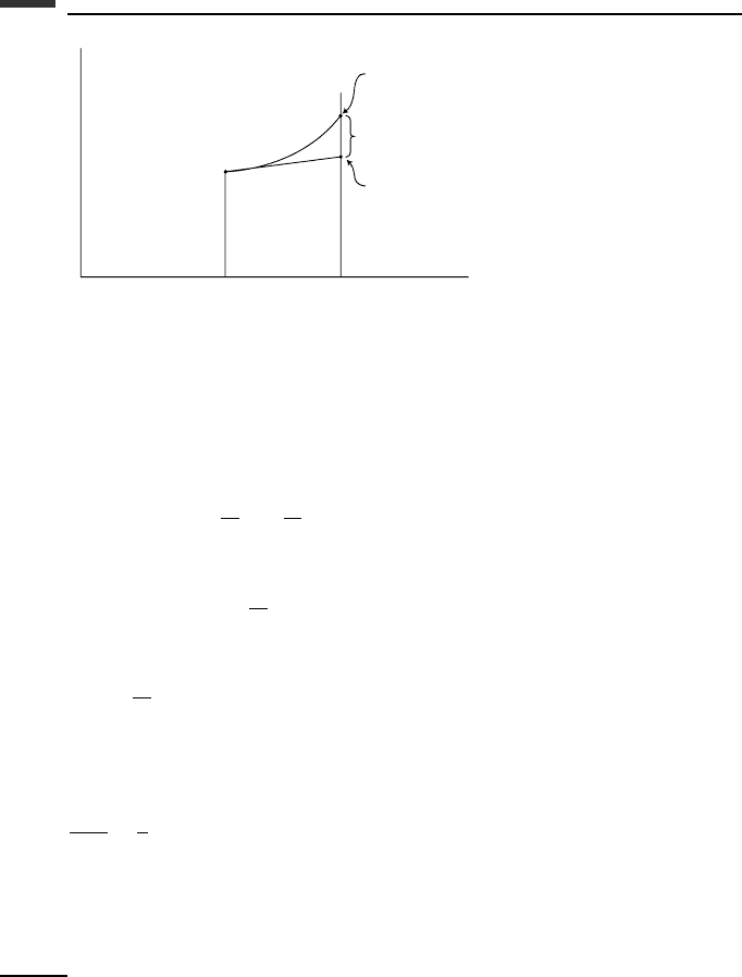
338 Introduction to numerical methods
y
n+1
(true value)
local truncation
error
y
*
n+1
(computed
value)
y
tt
n
y
n
t
n+1
Figure 6.2.
where
˙
y
n
= f (y
n
, t
n
) (6.62)
as shown in Fig. 6.2. To obtain the truncation error, consider a Taylor series about the time
t
n
,
y
n+1
= y
n
+ h
˙
y
n
+
h
2
2!
¨
y
n
+
h
3
3!
...
y
n
+··· (6.63)
The local truncation error can be approximated by the first error term, that is
E
n+1
= y
n+1
− y
∗
n+1
=
h
2
2!
¨
y
n
(6.64)
More accurately, using the mean value theorem, the local truncation error is
E
n+1
=
h
2
2!
¨
y(ξ )(t
n
<ξ<t
n+1
) (6.65)
for the Euler integration method.
Since the number of steps per unit time is inversely proportional to the step size h, and
assuming additive truncation errors, the corresponding global truncation error is
E
n+1
h
=
h
2
¨
y(ξ ) = O(h)(t
n
<ξ<t
n+1
) (6.66)
Because the global truncation error is of order h, the Euler method is called a first-order
method.
Roundoff errors
In addition to the truncation errors which are due to the numerical integration algorithm,
there are other errors which are due to the finite number of digits that are used in the
computations. These are called roundoff errors. A typical situation where roundoff errors
can become important occurs when the calculations involve the small difference of large