Gockenbach M.S. Partial Differential Equations. Analytical and Numerical Methods
Подождите немного. Документ загружается.

558
Appendix
C.
Solutions
to
odd-numbered
exercises
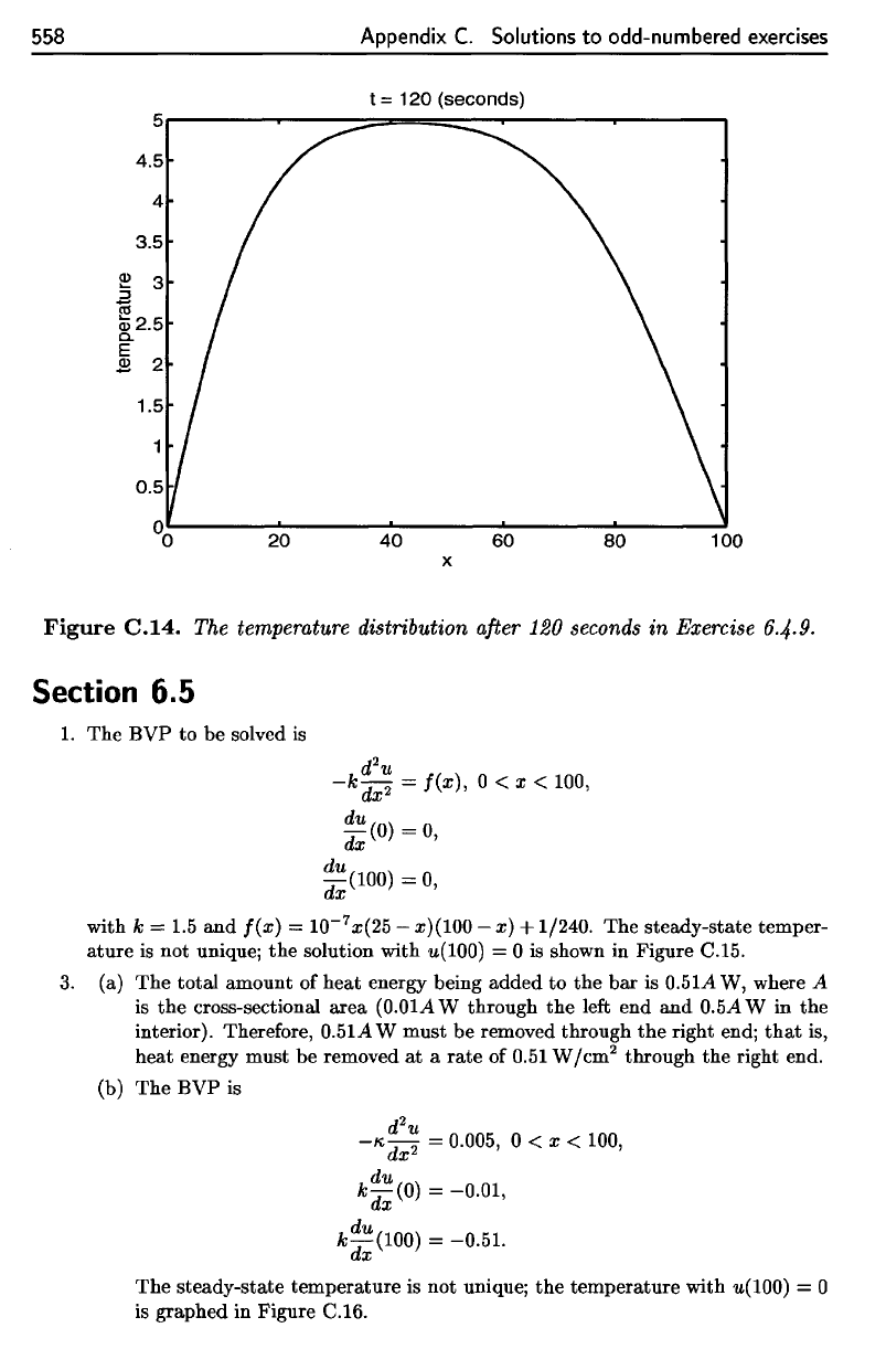
Figure
C.14.
The
temperature
distribution
after
120
seconds
in
Exercise
6.4-9.
Section
6.5
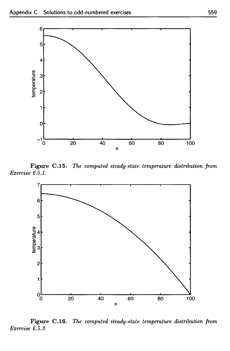
1.
The BVP to be
solved
is
with
k
=
1.5 and
f(x)
=
10~
7
x(25
-
z)(100
-
z)
+1/240.
The
steady-state
temper-
ature
is not
unique;
the
solution with
ii(100)
= 0 is
shown
in
Figure
C.15.
3.
(a) The
total
amount
of
heat energy being added
to the bar is
0.51A
W,
where
A
is
the
cross-sectional area
(0.01
AW
through
the
left
end and
0.5AW
in the
interior).
Therefore,
0.51
AW
must
be
removed through
the
right end;
that
is,
heat energy must
be
removed
at a
rate
of
0.51 W/cm
2
through
the
right end.
(b)
The BVP is
The
steady-state
temperature
is not
unique;
the
temperature with
w(100)
= 0
is
graphed
in
Figure
C.16.
558
Appendix
C.
Solutions
to
odd-numbered exercises
t =
120
(seconds)
5r-----~----~====~~~----~----__,
4.5
4
3.5
~
3
::::I
T!!
Q)2.5
c..
E
2 2
20
40
60
80
100
x
Figure
C.14.
The temperature distribution after 120 seconds in Exercise 6.4.9.
Section 6.5
1.
The
BVP
to
be solved
is
d
2
u
-k
dx
2
=
f(x),
0 < x < 100,
~:(O)
= 0,
du
(100) = 0,
dx
with k = 1.5
and
f(x)
= 1O-7
x
(25-x)(100-x)
+1/240.
The
steady-state temper-
ature
is not unique;
the
solution with u(100) = 0 is shown in Figure C.15.
3.
(a)
The
total amount of heat energy being
added
to
the
bar
is 0.51A W, where A
is
the
cross-sectional
area
(O.OlA
W through
the
left end
and
0.5A W in
the
interior). Therefore, 0.51A W
must
be removed through
the
right end;
that
is,
heat energy must be removed
at
a
rate
of 0.51 W
jcm
2
through
the
right end.
(b)
The
BVP
is
d
2
u
-I>,
dx
2
= 0.005, 0 < x < 100,
du
k dx
(0)
= -0.01,
du
k dx (100) =
-0.51.
The
steady-state
temperature
is not unique;
the
temperature
with u(100) = 0
is graphed in Figure C.16.
Appendix
C.
Solutions
to
odd-numbered exercises
559
Figure
C.I6.
The
computed steady-state temperature distribution from
Exercise 6.5.3.
Figure
C.I5.
The
computed steady-state temperature distribution
fron
J^.fOTfnoo
fi
t\
1
Appendix
C.
Solutions
to
odd-numbered exercises
6r-------~------_r------~--------r_------~
5
4
Q)
::;
3
"§
Q)
a.
E 2
2
o
-1~------~------~------~--------~----~
o
20
40
60 80
100
x
559
Figure
C.15.
The computed steady-state temperature distribution from
Exercise
6.5.1.
7~------~------~--------~------~-------,
6
5
2
°o~------~------~------~------~----~
20
40
60
80
100
x
Figure
C.16.
The computed steady-state temperature distribution from
Exercise 6.5.3.
560
Appendix
C.
Solutions
to
odd-numbered
exercises
5.
(a) We
have
Therefore,
(b)
Suppose
v
G
V and
a(v,
v) = 0. By
definition
of
a(-,
•),
this
is
equivalent
to
Since
the
integrand
is
nonnegative,
this
implies
that
the
integrand
is in
fact
zero,
and, since
K(X)
is
positive,
we
conclude
that
is
the
zero function. Therefore,
v is a
constant
function,
(c)
Thus,
if
Ku
= 0, it
follows
that
is a
constant
function,
where
MO,
1*2,
• •
•,
u
n
are the
components
of u. But
then
there
is a
constant
C
such
that
v(xi)
— C, i =
0,1,
2,...,
n.
These nodal
values
of v are
precisely
the
numbers
UQ,
MI,
...,u
n
,
so we see
that
u =
Cu
c
,
which
is
what
we
wanted
to
prove.
7.
(a)
Define
Then
the
weak
form
of the BVP is
(b)
The
fact
that
a
solution
of the
strong
form
is
also
a
solution
of the
weak
form
is
proved
by the
usual argument: multiply
the
differential
equation
by an
arbitrary
test
function
v €
V",
and
then
integrate
by
parts.
560
Appendix
C.
Solutions
to
odd-numbered
exercises
5.
(a) We have
7.
Therefore,
n n
u·Ku=
LLK;jUjU;
i=O
j=O
n n
= L
La
(4)j,
4>i)
UjU;
i=O
j=O
~
t,a
(t,
.;f;,f}
~
a
(t,
.;~;,
t,
.;~;)
=a(v,v).
Ku
= 0
~
U·
Ku
= 0
~
a(v,v)
=
o.
(b) Suppose v E
iT
and
a( v, v) =
O.
By definition of a(-, .), this is equivalent
to
Since
the
integrand is nonnegative, this implies
that
the
integrand is in fact
zero, and, since
K(X)
is positive,
we
conclude
that
dv(X)
dx
is
the
zero function. Therefore, v is a constant function.
(c) Thus, if
Ku
=
0,
it
follows
that
n
v(X) = L
U;4>i(X)
;=0
is a constant function, where
Uo,
U2,
.
..
,
Un
are
the
components of
u.
But
then
there is a constant C such
that
V(Xi)
= C, i = 0,1,2,
...
, n. These nodal
values of
v are precisely
the
numbers
Uo,
Ul,
...
,
Un,
so
we
see
that
u =
CUe,
which is
what
we
wanted
to
prove.
(a) Define
v(O)
=
O}.
Then
the
weak form of
the
BVP
is
find
U E V such
that
a(u, v) = (I, v) for all v E
V.
(CA)
(b)
The
fact
that
a solution of
the
strong form is also a solution of
the
weak
form is proved by
the
usual argument: multiply
the
differential equation by an
arbitrary
test
function v E
V,
and
then
integrate
by
parts.
Appendix
C.
Solutions
to
odd-numbered
exercises
561
The
proof
that
a
solution
of the
weak
form
is
also
a
solution
of the
strong
form
is
similar
to the
argument given
on
page 268. Assuming
that
u
satisfies
the
weak
form
(C.4),
an
integration
by
parts
and
some simplification shows
that
Since
V C
V,
this
implies
that
the
differential
equation
holds,
and we
then have
Choosing
any v € V
with
v(i}
^
0
shows
that
the
Neumann condition holds
at x
—
t.
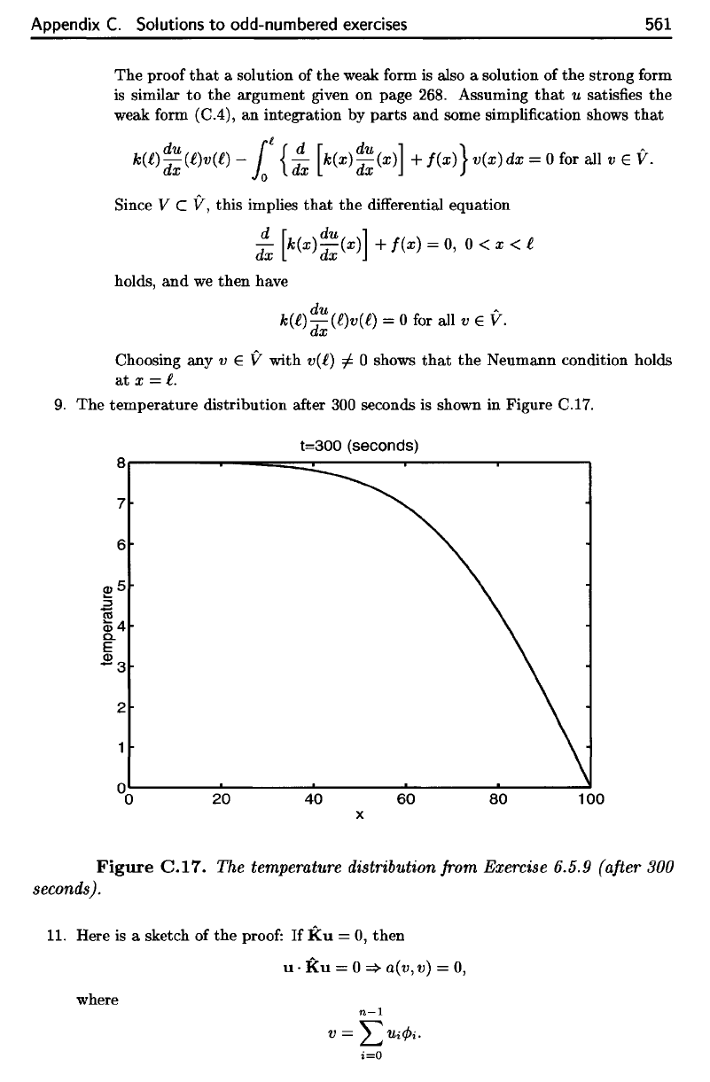
9.
The
temperature
distribution after
300
seconds
is
shown
in
Figure
C.I7.
Figure
C.I7.
The
temperature distribution from Exercise 6.5.9
(after
300
seconds).
11.
Here
is a
sketch
of the
proof:
If
Ku
= 0,
then
where
Appendix
C.
Solutions
to
odd-numbered exercises
561
The
proof
that
a solution of
the
weak form is also a solution of
the
strong form
is similar
to
the
argument given on page
268.
Assuming
that
U satisfies
the
weak form (C.4), an integration by
parts
and
some simplification shows
that
k(£)
~:
(£)v(£)
-1£
{:x
[k(X)
~:
(x)] +
f(x)}
v(x) dx = 0 for all v E
V.
Since V C
V,
this implies
that
the
differential equation
d [ du ]
dx
k(x)dx(x)
+f(x)=O,
O<x<£
holds,
and
we
then
have
du •
k(£) dx (£)v(£) = 0 for all v E
V.
Choosing any v E V with v(£)
f::.
0 shows
that
the
Neumann condition holds
at
x =
£.
9.
The
temperature
distribution after 300 seconds is shown in Figure C.17.
t=300
(seconds)
8r-----------==~~-----r------~------,
7
6
2
20
40
60
80
100
x
Figure
C.17.
The temperature distribution from Exercise 6.5.9 {after 300
seconds}.
11. Here is a sketch of
the
proof:
If
Ku
= 0,
then
u·
Ku
= 0
=>
a(v, v) =
0,
where
n-l
V = LUi¢>i.
;=0
562
Appendix
C.
Solutions
to
odd-numbered
exercises
But
then,
by the
usual reasoning,
v
must
be a
constant
function,
and
v(x
n
)
= 0
(since
(j)i(x
n
)
= 0 for i =
0,1,
2,...,
n
—
1).
Thus
v is the
zero
function,
which implies
that
the
nodal values
of v are all
zero. Therefore
u = 0, and so
K
is
nonsingular.
Section
6.6
1.
For t =
6060,
only
2
terms
are
required
for an
accurate graph, while
for t = 61,
about
150
terms
are
required.
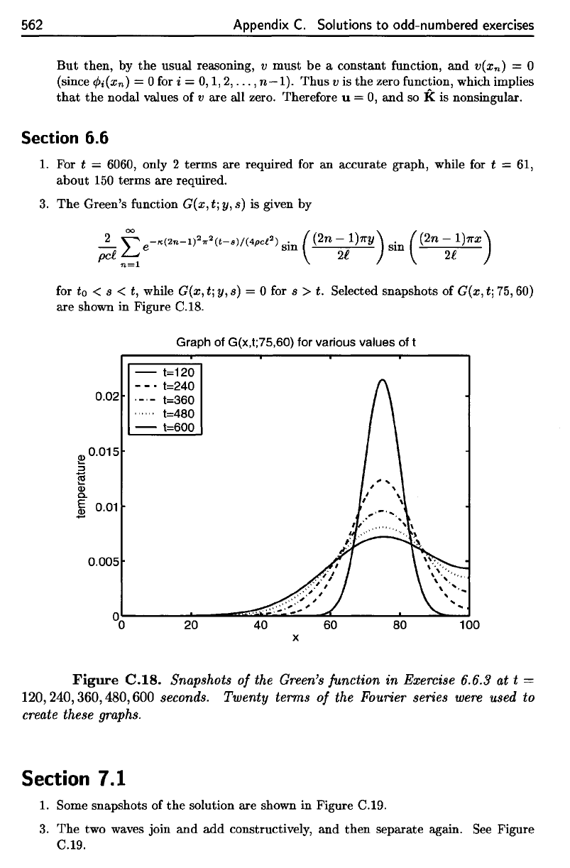
3. The
Green's
function
G(a;,t;r/,s)
is
given
by
for
to < s <
t,
while
G(x,
t;
y, s) = 0 for s > t.
Selected snapshots
of
G(x,
t]
75,60)
are
shown
in
Figure
C.I8.
Graph
of
G(x,t;75,60)
for
various values
of t
Figure
C.18.
Snapshots
of
the
Green's
function
in
Exercise
6.6.3
at t =
120,240,360,480,600
seconds.
Twenty
terms
of the
Fourier
series
were
used
to
create
these
graphs.
Section
7.1
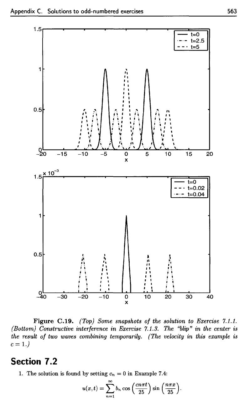
1.
Some snapshots
of the
solution
are
shown
in
Figure
C.19.
3. The two
waves join
and add
constructively,
and
then
separate
again.
See
Figure
C.19.
562
Appendix
C.
Solutions
to
odd-numbered exercises
But
then, by
the
usual reasoning, v
must
be a constant function,
and
V(Xn)
= 0
(since
CPi(X
n
)
= 0 for i =
0,1,2,
...
,
n-l).
Thus v is
the
zero function, which implies
that
the
nodal values of v are all zero. Therefore u =
0,
and
so
K is nonsingular.
Section 6.6
1. For t = 6060, only 2 terms are required for an accurate graph, while for t = 61,
about
150 terms are required.
3.
The
Green's function G(x,
t;
y,
s)
is given by
2
~
-K(2n-l)2,,2(t-8)/(4pcl
2
) .
((2n
-1)1r
Y) .
((2n
-1)1rX)
~~e
~
U
~
U
n=l
for
to
< s < t, while G(x,
t;
y,
s)
= 0 for s > t. Selected snapshots of G(x,
t;
75, 60)
are shown in Figure C.18.
Graph of G(x,t;75,60) for various values of t
- t=120
-
_.
t=240
0.02
._,-
t=360
~
0.015
:::l
"@
<D
Cl.
E 0.01
$
0.005
'"''
t=480
- t=600
20 40
60 80
x
100
Figure
C.IS.
Snapshots
of
the Green's function
in
Exercise 6.6.3 at t =
120,
240,
360, 480, 600 seconds. Twenty terms
of
the Fourier series were used to
create these graphs.
Section 7.1
1. Some snapshots of
the
solution are shown in Figure C.19.
3.
The
two waves join
and add
constructively,
and
then
separate again. See Figure
C.19.
Appendix
C.
Solutions
to
odd-numbered exercises
563
Figure
C.19.
(Top)
Some snapshots
of the
solution
to
Exercise 7.1.1.
(Bottom) Constructive interference
in
Exercise 7.1.3.
The
"blip"
in the
center
is
the
result
of two
waves combining temporarily.
(The
velocity
in
this example
is
c
=
l.)
Section
7.2
1.
The
solution
is
found
by
setting
c
n
= 0 in
Example 7.4:
Appendix
C.
Solutions
to
odd-numbered exercises
1.5.--.-----r--.....---.....--.----.-r========i1
t=o
t=2.5
t=5
1\
,
"
"
"
"
, ,
,
,
I
I
,
,
I
I
, ,
,
...
~
1&
I I
."
, I _ ,
,.'
I I
~
..
"
~"
f , I I "
, ' , - - - I -
I;~
~~,
~!~
I I i
~
r'
I
l~!
~i
~
~"
..
~
0.5
..
1\
ii
I I
,
I
,
I
I
,
I
•
- ,
~
I.
I.
•
I),
j\
'\
/'j'
OL-____
~
__
6_~~/~\~~-~J_'\~/_~,-~I_\~_'~~~~~~
__
~
____
~
'\.
.,
I I -
,
15
-20 -15 -10
-5
0
-3
1.5
x
10
0.5
-~O
-30
!
i
'
"
, I
•
,
-20
x
I
"
'I
• I
,
I
•
I
,
I
I
-10
0
x
5
"
"
"
I I
,
I
,
I
,
I
,
I
I
10
10
I
i
,-
-I
,-
,!
i I
i !
i
!
,
I
20
t=O
t=0.02
t=0.04
30
20
40
563
Figure
C.19.
(Top) Some snapshots
of
the solution to Exercise 7.1.1.
(Bottom) Constructive interference in Exercise
7.1.3. The "blip" in the center is
the result
of
two waves combining temporarily. (The velocity in this example is
c = 1.)
Section 7.2
1.
The
solution is found
by
setting
en = 0 in Example 7.4:
~
(cn7rt)
.
(n7rx)
u(x,t)
=
~bncos
~
sm
25
.
n=l
564
Appendix
C.
Solutions
to
odd-numbered
exercises
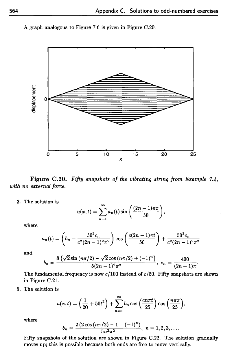
A
graph analogous
to
Figure
7.6 is
given
in
Figure
C.20.
Figure
C.20.
Fifty
snapshots
of the
vibrating string from Example
7-4,
with
no
external force.
3.
The
solution
is
where
and
where
Fifty
snapshots
of the
solution
are
shown
in
Figure
C.22.
The
solution gradually
moves
up;
this
is
possible because both ends
are free to
move vertically.
The
fundamental
frequency is now
c/100
instead
of
c/50.
Fifty
snapshots
are
shown
in
Figure C.21.
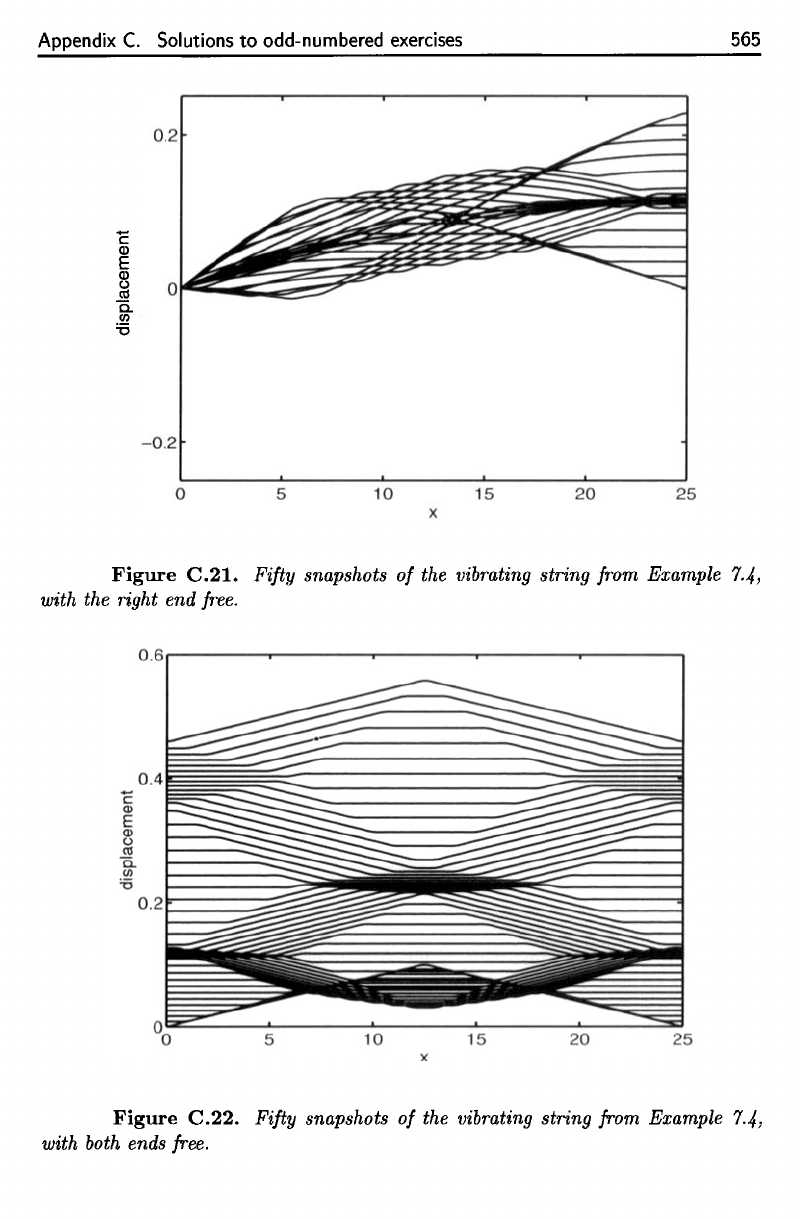
5.
The
solution
is
564
Appendix
C.
Solutions
to
odd-numbered exercises
A graph analogous
to
Figure 7.6 is given in Figure C.20.
o 5
10
15
20
25
x
Figure
C.20.
Fifty snapshots
of
the vibrating string from Example 7.4,
with no external force.
3.
The
solution is
00
•
(2n-1)1I'X)
u(X,t) =
Lan(t)sm
50
'
n=l
where
and
8
(v'2sin
(n1l'/2)
-
v'2cos
(n1l'/2)
+ (_1)n)
400
b
n
= ,en= .
5(2n -
1)211'2
(2n -
1)11'
The
fundamental frequency is now c/100 instead of c/50. Fifty snapshots are shown
in Figure C.2l.
5.
The
solution is
(
1
2)
~
(cn1l't) (n1l'X)
u(x,t)
=
20
+50t
+
~bncos
25
cos
25
'
where
n=l
b
n
=
2(2cos(n1l"2~
~
1-
(-It),
n =
1,2,3,
....
n1l'
Fifty snapshots of
the
solution are shown in Figure C.22.
The
solution gradually
moves up; this is possible because
both
ends are free
to
move vertically.
Appendix
C.
Solutions
to
odd-numbered
exercises
565
Figure
C.21.
Fifty
snapshots
of the
vibrating
string
from Example
7.4,
with
the
right
end
free.
Figure
C.22.
Fifty
snapshots
of the
vibrating string from Example
7.4,
with
both ends free.
Appendix
C.
Solutions
to
odd-numbered exercises
c
CD
E
CD
~
'i5..
In
'i5
0
.2
- 0.2
o 5
10
x
565
15
20
25
Figure
C.21.
Fifty snapshots
of
the vibrating string from Example 7.4,
with the right end
free.
'E
CD
E
CD
<..>
<II
a.
0.2
5
10
15
20
25
x
Figure
C.22.
Fifty snapshots
of
the vibrating string from Example 7.4,
with both ends free.
566
Appendix
C.
Solutions
to
odd-numbered
exercises
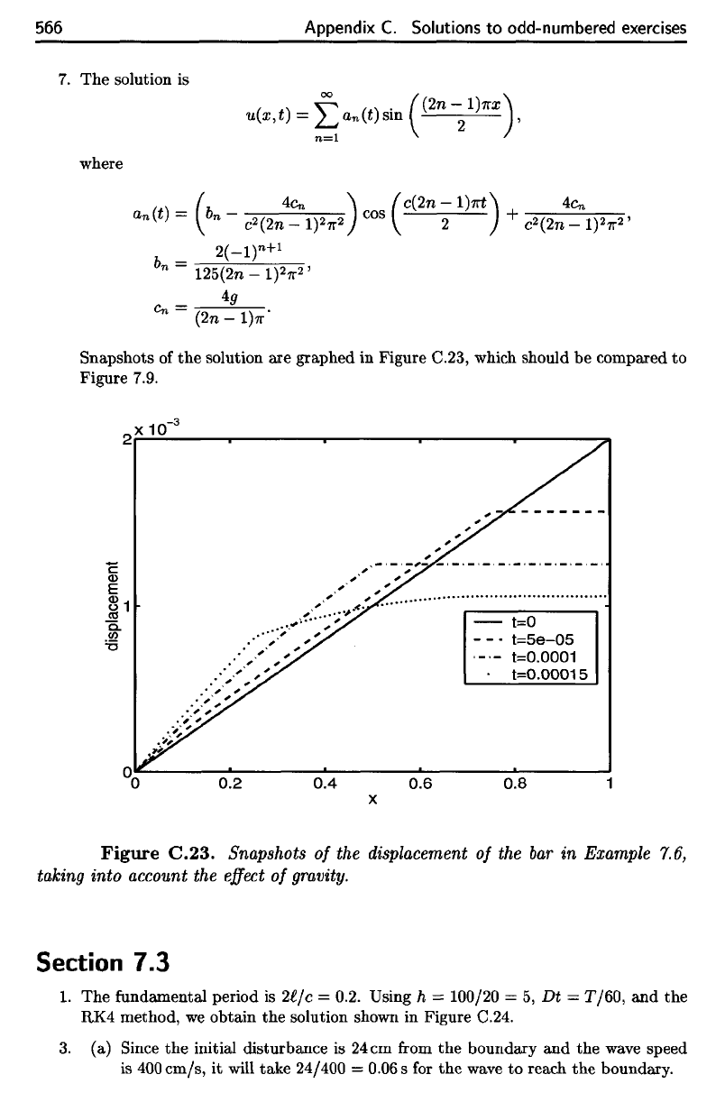
7.
The
solution
is
where
Snapshots
of the
solution
are
graphed
in
Figure
C.23,
which should
be
compared
to
Figure 7.9.
Figure
C.23. Snapshots
of the
displacement
of the bar in
Example 7.6,
taking
into
account
the
effect
of
gravity.
Section
7.3
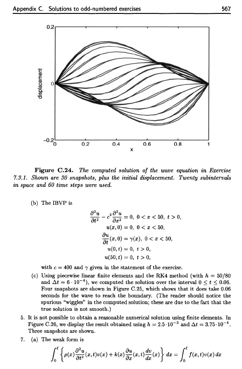
1.
The
fundamental period
is
li/c
=
0.2. Using
h =
100/20
=
5,
Dt =
T/60,
and the
RK4
method,
we
obtain
the
solution shown
in
Figure
C.24.
3.
(a)
Since
the
initial disturbance
is
24cm
from
the
boundary
and the
wave speed
is
400cm/s,
it
will take 24/400
=
0.06s
for the
wave
to
reach
the
boundary.
566
Appendix
C.
Solutions
to
odd-numbered exercises
7.
The
solution is
where
00
•
(2n-1)1rX)
u(x, t) =
~
an(t) sm 2 '
an(t) =
(bn-
C2(2n4~1)21r2)cos(C(2n;1)1rt)
+
c2(2n4~1)21r2'
2(_1)n+l
b
n
= 125(2n -
1)21r
2
'
4g
en
= -,-----"--:--
(2n -
1)1r
Snapshots of
the
solution are graphed in Figure C.23, which should
be
compared
to
Figure 7.9.
,-
-
-,
-,_._,-
- _._,-,-,-
-,
; ;
; ;
""
,,'
........................................
.
....
.
;.,.;:~:~
..
-;~
....
- t=O
-
_.
t=5e-05
0°
,.
. ' ;
. ; ;
.....
>;>'
.-:>;"
.,
;
.0,'
,
t=0.0001
t=0.00015
.--';'
;{'-
°o~------~------~------~------~------~
0.2
0.4 0.6 0.8
x
Figure
C.23.
Snapshots
of
the displacement
of
the
bar
in Example
7.6,
taking into account the effect
of
gravity.
Section 7.3
1.
The
fundamental period
is
2l/c
= 0.2. Using h = 100/20 =
5,
Dt
=
T/60,
and
the
RK4
method,
we
obtain
the
solution shown in Figure C.24.
3.
(a) Since
the
initial disturbance is
24cm
from
the
boundary
and
the
wave speed
is 400
cm/s,
it
will
take
24/400 = 0.06 s for
the
wave
to
reach
the
boundary.
Appendix
C.
Solutions
to
odd-numbered
exercises
567
Figure
C.24.
The
computed
solution
of the
wave equation
in
Exercise
7.3.1.
Shown
are 30
snapshots,
plus
the
initial
displacement. Twenty subintervals
in
space
and 60
time
steps were used.
(b)
The
IBVP
is
with
c = 400 and 7
given
in the
statement
of the
exercise.
(c)
Using
piecewise
linear
finite
elements
and the RK4
method (with
h =
50/80
and
At
= 6 •
10~
4
),
we
computed
the
solution over
the
interval
0
<
t
<
0.06.
Four
snapshots
are
shown
in
Figure
C.25,
which shows
that
it
does take 0.06
seconds
for the
wave
to
reach
the
boundary. (The reader should notice
the
spurious
"wiggles"
in the
computed solution; these
are due to the
fact
that
the
true solution
is not
smooth.)
5.
It is not
possible
to
obtain
a
reasonable numerical solution using
finite
elements.
In
Figure
C.26,
we
display
the
result obtained using
h —
2.5-10~
3
and
At
=
3.75-10~
4
.
Three snapshots
are
shown.
7.
(a) The
weak
form
is
Appendix
C.
Solutions
to
odd-numbered exercises
'E
Q)
E
g
Ci
<IJ
'6
O
.
2
r-------~-------,--------~------~------~
-
0
.
2
~------~--------~------~--------~------~
o 0.2 0.4 0.6 0.8
x
567
Figure
C.24.
The computed solution
of
the wave equation in Exercise
7.3.1. Shown
are
30 snapshots, plus the initial displacement. Twenty subintervals
in space and
60
time steps were used.
(b)
The
IBVP
is
a
2
u 2 a
2
u
at
2
-
c ax
2
=
0,
0 < x <
50,
t >
0,
u(x,O) =
0,
0 < x <
50,
au
at
(x,O)
=
,(x),
0 < x <
50,
u(O,
t) = 0, t > 0,
u(50, t) =
0,
t >
0,
with c = 400
and
, given in
the
statement
of
the
exercise.
(c) Using piecewise linear finite elements
and
the
RK4
method
(with h = 50/80
and
.6.t
= 6 .
10-
4
),
we
computed
the
solution over
the
interval 0
~
t
~
0.06.
Four snapshots are shown in Figure
C.25, which shows
that
it does take 0.06
seconds for
the
wave
to
reach
the
boundary. (The reader should notice
the
spurious "wiggles" in
the
computed solution; these are due
to
the
fact
that
the
true
solution is not smooth.)
5.
It
is not possible
to
obtain a reasonable numerical solution using finite elements.
In
Figure C.26,
we
display
the
result obtained using h =
2.5.10-
3
and
.6.t
=
3.75.10-
4
•
Three snapshots are shown.
7.
(a)
The
weak form is
1
£
{a
2
u
au
dV}
It
o p(x)
(Jt2
(x, t)v(x) + k(x) ax (x, t)
dx
(x)
dx
= 0
f(x,
t)v(x)
dx