Gockenbach M.S. Partial Differential Equations. Analytical and Numerical Methods
Подождите немного. Документ загружается.

398
Chapter
9.
More about Fourier
series
9.1.4
The
complex Fourier
series
of a
real-valued function
If
/ €
C[—i,i]
is
real-valued,
then, according
to our
assertions above,
it can be
represented
by its
complex Fourier series.
We now
show
that,
since
/ is
real-valued,
each
partial
sum
(n
=
—TV,
—
JV
+
1,...,
AT)
of the
complex Fourier series
is
real,
and
moreover
that
the
complex Fourier series
is
equivalent
to the
full
Fourier series
in
this
case.
So
we
suppose
/ is
real-valued
and
that
c
n
,
n = 0, ±1,
±2,...
are its
complex
Fourier
coefficients.
For
reference,
we
will
write
the
full
Fourier series
of /
(see
Section
6.3)
as
where
Now,
For
n > 0,
Similary,
with
n > 0, we
have
398 Chapter 9. More about Fourier series
9.1.4 The complex Fourier
series
of a real-valued function
If
f E
C[
-e,
e]
is
real-valued, then, according to our assertions above,
it
can be
represented by its complex Fourier series.
We
now show
that,
since f
is
real-valued,
each partial sum
(n =
-N,
-N
+ 1,
...
,
N)
of
the
complex Fourier series
is
real,
and moreover
that
the
complex Fourier series
is
equivalent
to
the
full Fourier series
in this case.
So
we
suppose f
is
real-valued and
that
Cn,
n = 0,
±1, ±2,
...
are its complex
Fourier coefficients. For reference,
we
will write the full Fourier series of f (see
Section
6.3) as
where
Now,
For
n > 0,
00
ao
+ L (an
cos
(n;x)
+ b
n
sin
(n;x))
,
n=l
1
1£
ao
= 2f
f(x)
dx,
-l
11£
(n7rx)
an
="£
f(x)cos
-e- dx, n =
1,2,3,
...
,
-£
11£
. (n7rx)
b
n
="£
f(x)sm
-e- dx, n =
1,2,3,
....
-£
1
II
Co
= 2f
f(x)
dx =
ao·
-l
C
n
=
2~
ill
f(x)e-i7rnx/l dx
=
;e
ill
f(x)
(cos
(n;x)
- i sin
(n;x))
dx
=
;e
ill
f(x)
cos
(n;x)
dx -
;e
ill
f(x)
sin
(n;x)
dx
1 i
= 2
an
- 2
bn
.
Similary, with n >
0,
we
have
C-
n
=
;e
[ll
f(x)ei7rnx/l dx
=
;e
[i/(X)
(cos
(n;x)
+isin
(n;x))
dx
=
;e
[le
f(x)
cos
(n;x)
dx +
;e
[:
f(x)
sin
(n;x)
dx
9.1.
The
complex Fourier
series
399
Therefore,
(The reader should notice
how all
imaginary quantities
sum to
zero
in
this calcula-
tion.)
Therefore,
for
any
N > 0,
This shows
that
every (symmetric)
partial
sum of the
complex Fourier series
of a
real-valued
function
is
real
and
also
that
the
complex Fourier series
is
equivalent
to
the
full
Fourier series.
Exercises
1.
Let / :
[-1,1]
->•
R be
defined
by
f(x)
=
I
—
x
2
.
Compute
the
complex
Fourier series
of
/, and
graph
the
errors
for
TV
=
10,20,40.
2.
Let / :
[—7r,7r]
—>•
R be
denned
by
f(x)
= x.
Compute
the
complex Fourier
coefficients
c
n
,
n
= 0, ±1,
±2,...,
of /, and
graph
the
errors
for
TV
=
10,20,40.
3.
Let / :
[—1,1]
—>
C be
defined
by
f(x)
=
e
lx
.
Compute
the
complex Fourier
coefficients
c
n
,
n
—
0, ±1,
±2,...,
of /, and
graph
the
errors
9.1.
The
complex
Fourier
series 399
Therefore,
cnei7rnx/£
+ c_ne-i7rnx/l =
(~an
_
~bn
) (cos
(n;x)
+ i sin
(n;x))
+
(~an+~bn)
(cos
(n;x)
_isin(n;x))
= an
cos
(n;x)
+ b
n
sin
(n;x).
(The reader should notice how all imaginary quantities sum to zero in this calcula-
tion.)
Therefore, for any
N 2
0,
N N
L
Cnei7rnx/l
=
ao
+ L
(an
cos
(n;x)
+ b
n
sin
(n;x))
.
n=-N
n=1
This shows
that
every (symmetric) partial sum of
the
complex Fourier series of a
real-valued function
is
real and also
that
the complex Fourier series
is
equivalent
to
the
full Fourier series.
Exercises
1.
Let f :
[-1,1]
-+
R be defined by
f(x)
= 1 - x
2
.
Compute the complex
Fourier series
of
f, and graph the errors
N
f(x)
- L
cnei7rnx
n=-N
for N = 10,20,40.
2.
Let f :
[-71",71"]
-+ R be defined by
f(x)
=
x.
Compute
the
complex Fourier
coefficients
Cn,
n =
0,
±1,
±2,
...
, of
j,
and graph the errors
N
f(x)
- L cne
inx
n=-N
for N = 10,20,40.
3.
Let f:
[-1,1]-+
C be defined by
f(x)
= e
ix
. Compute the complex Fourier
coefficients
Cn,
n =
0,
±1, ±2,
...
, of f, and graph the errors
N
f(x)
- L c
n
e
i
7l"nx
n=-N
400
Chapter
9.
More about Fourier
series
for
N
=
10,20,40.
(Note:
You
will
have
to
either graph
the
real
and
imaginary
parts
of the
error separately
or
just graph
the
modulus
of the
error.)
4.
Consider
the
negative second derivative operator under periodic boundary
conditions
on
[—£,•£].
(a)
Show
that
each pair listed
in
(9.2)
is an
eigenpair.
(b)
Show
that
(9.2) includes
every
eigenvalue.
(c)
Show
that
every
eigenfunction
is
expressible
in
terms
of
those given
in
(9.2).
(d)
Compare these results
to
those derived
in
Section 6.3,
and
explain
why
they
are
consistent.
5.
Suppose
that
/ :
[—•£,•£]
—>
C is
defined
by
f(x)
=
g(x]
+
ih(x),
where
g and
h are
real-valued
functions
defined
on
[—i,£].
Show
that
the
complex Fourier
coefficients
can be
expressed
in
terms
of the
full
Fourier
coefficients
of g and
h.
6.
Prove
that,
for any
real numbers
0 and A,
(Hint:
Use
Euler's
formula
and
trigonometric identities.)
7. Let
TV
be a
positive integer,
j a
positive
integer
between
1 and N
—
1, and
define
vectors
u
e
R
N
and v
e
R
N
by
\ / \
/
(For
this exercise,
it is
convenient
to
index
the
components
of x €
R
N
as
0,1,...,
TV
—
1,
instead
of
1,2,...,
TV
as is
usual.)
The
purpose
of
this exercise
is
to
prove
that
(a)
u • v = 0,
that
is, u and v are
orthogonal.
These results
are
based
on the
following
trick:
The sum
is
a finite
geometric series,
for
which there
is a
simple
formula.
On the
other
hand.
can be
rewritten
by
replacing
e
7r
'
l
J
n
/
N
by cos
(jnir/N)
+i sin
(jrnr/N),
expand-
ing
the
square,
and
summing. Find
the sum
(9.3) both ways,
and
deduce
the
results given above.
400
Chapter 9. More
about
Fourier series
for N = 10,20,40. (Note:
You
will have
to
either graph the real and imaginary
parts
of
the
error separately or
just
graph the modulus of
the
error.)
4.
Consider
the
negative second derivative operator under periodic boundary
conditions on
[-f,f].
(a) Show
that
each pair listed in (9.2)
is
an
eigenpair.
(b) Show
that
(9.2) includes every eigenvalue.
(c) Show
that
every eigenfunction
is
expressible in terms of those given in
(9.2).
(d) Compare these results
to
those derived in Section 6.3, and explain why
they are consistent.
5.
Suppose
that
f:
[-f,f]
~
C
is
defined by
f(x)
= g(x)
+ih(x),
where 9 and
h are real-valued functions defined on
[-f,f].
Show
that
the complex Fourier
coefficients can be expressed in terms of
the
full Fourier coefficients of 9 and
h.
6.
Prove
that,
for any real numbers
()
and
>.,
ei(II+>') = e
i
()
e
i
>..
(Hint: Use Euler's formula and trigonometric identities.)
7.
Let N be a positive integer, j a positive integer between 1 and N - 1, and
define vectors u
ERN
and
v
ERN
by
(
jn~)
.
(jn~)
Un
= cos N
,V
n
=
SIn
N
,n
=
0,1,
...
,N
- 1.
(For this exercise,
it
is
convenient
to
index the components of x E
RN
as
0,
1,
...
,N
-
1,
instead of 1,2,
...
, N as
is
usual.) The purpose of this exercise
is
to
prove
that
(a)
u·
v =
0,
that
is, u and v are orthogonal.
(b)
Ilull
=
IIvll
= IN/2.
These results are based on
the
following trick: The sum
N-l
2
N-I
L
(e1fijn/N)
= L
(e
21fij
/
N
f
n=O
n=O
is a finite geometric series, for which there
is
a simple formula. On
the
other
hand,
N-I
2
L
(e1fijn/N)
(9.3)
n=O
can be rewritten by replacing
e1fijn/N
by cos
(jn~/N)+i
sin
(jn~/N),
expand-
ing
the
square, and summing. Find the sum (9.3) both ways, and deduce the
results given above.
9.2.
Fourier
series
and the FFT
401
9.2
Fourier
series
and the FFT
We
now
show
that
there
is a
very
efficient
way to
estimate Fourier
coefficients
and
evaluate (partial) Fourier series.
We
will
use the BVP
as our first
example.
To
solve this
by the
method
of
Fourier series,
we
express
u
and
/ in
complex Fourier series,
say
(c
n
,
n
=
0, ±1,
±2,...
unknown)
and
(d
n
,n
=
0,±l,±2,...
known).
The
differential
equation
can
then
be
written
as
and we
obtain
The
reader
will
notice
the
similarity
to how the
problem
was
solved
in
Section
6.3.2. (The calculations, however,
are
simpler when using
the
complex Fourier
series
instead
of the
full
Fourier series.)
As in
Section 6.3.2,
the
coefficient
do
must
be
zero,
that
is,
must hold,
in
order
for a
solution
to
exist. When this compatibility condition holds,
the
value
of
CQ
is not
determined
by the
equation
and
infinitely
many solutions exist,
differing
only
in the
choice
of
c
0
.
For
analytic purposes,
the
formula
(9.6)
may be all we
need.
For
example,
as
we
discuss
in
Section 9.5.1, (9.6) shows
that
the
solution
u is
considerably smoother
than
the
forcing
function
/
(since
the
Fourier
coefficients
of u
decay
to
zero faster
than
those
of
/).
However,
in
many
cases,
we
want
to
produce
a
numerical
estimate
of
the
solution
u. We may
wish,
for
example,
to
estimate
the
values
of u on a
grid
so
that
we can
graph
the
solution accurately. This requires three steps:
9.2. Fourier series and
the
FFT
401
9.2 Fourier
series
and
the FFT
We
now show
that
there
is
a very efficient way
to
estimate Fourier coefficients
and
evaluate (partial) Fourier series.
We
will use the
BVP
cf2u
-K,-
=
f(x)
-£
< x < £
dx
2
,-
,
u(
-e)
=
u(£),
(9.4)
du(_£) = du(£)
dx dx
as our first example. To solve this by the method of Fourier series,
we
express u
and f in complex Fourier series, say
00
u(x) =
n=-oo
(en,
n =
0,
±1, ±2,
...
unknown) and
00
f(x)
= L
dnei7rnx/f
n=~oo
(d
n
,
n =
0,
±1, ±2,
...
known). The differential equation can
then
be written as
00
22
00
'""'
K,n
1f
c
ei7rnx/f
=
'""'
d
ei7rnx/f
~
£2
n
~n,
(9.5)
n=-oo
n=-oo
and
we
obtain
(9.6)
The reader will notice the similarity to how
the
problem was solved in Section
6.3.2. (The calculations, however, are simpler when using
the
complex Fourier
series instead of
the
full Fourier series.) As in Section 6.3.2,
the
coefficient
do
must
be zero,
that
is,
1
f
f(x)
dx = 0
~f
must hold, in order for a solution
to
exist. When this compatibility condition holds,
the
value of
Co
is not determined by
the
equation and infinitely many solutions exist,
differing only in the choice of
Co.
For analytic purposes, the formula (9.6) may
be
all
we
need. For example, as
we
discuss in Section 9.5.1, (9.6) shows
that
the
solution u is considerably smoother
than
the forcing function f (since the Fourier coefficients of u decay
to
zero faster
than
those of
f).
However, in many cases,
we
want
to
produce a numerical estimate
of the solution
u.
We
may wish, for example, to estimate the values of u on a grid
so
that
we
can graph the solution accurately. This requires three steps:
402
Chapter
9.
More
about
Fourier
series
1.
Compute
the
Fourier
coefficients
d
n
,
n
= 0, ±1,
±2,...,
TV,
of / by
evaluating
the
appropriate integrals.
2.
Compute
the
Fourier
coefficients
c
n
,
n = 0, ±1,
±2,...,
TV,
of u
from
formula
(9.6).
3.
Evaluate
the
partial
sum
on a
grid covering
the
interval
[—I,
I],
say Xj —
jh,
j = 0,
±1,±2,...
,±JV,
/i
=
£/JV.
If
JV
is
chosen large enough, this
will
produce accurate estimates
of
u(xj),
j —
0,±1,±2,...,±JV.
Until
this point,
we
have implicitly assumed
that
all of the
calculations nec-
essary
to
compute
u
would
be
done analytically (using various integration rules
to
compute
the
necessary Fourier
coefficients,
for
example). This
is not
always possi-
ble
(some integrals cannot
be
computed using elementary
functions)
and not
always
desirable when
it is
possible (because there
may be
more
efficient
methods).
We
will
therefore consider
how to
estimate
u.
9.2.1
Using
the
trapezoidal
rule
to
estimate
Fourier
coefficients
We
begin
by
estimating
the
integrals
defining
the
Fourier
coefficients
of /:
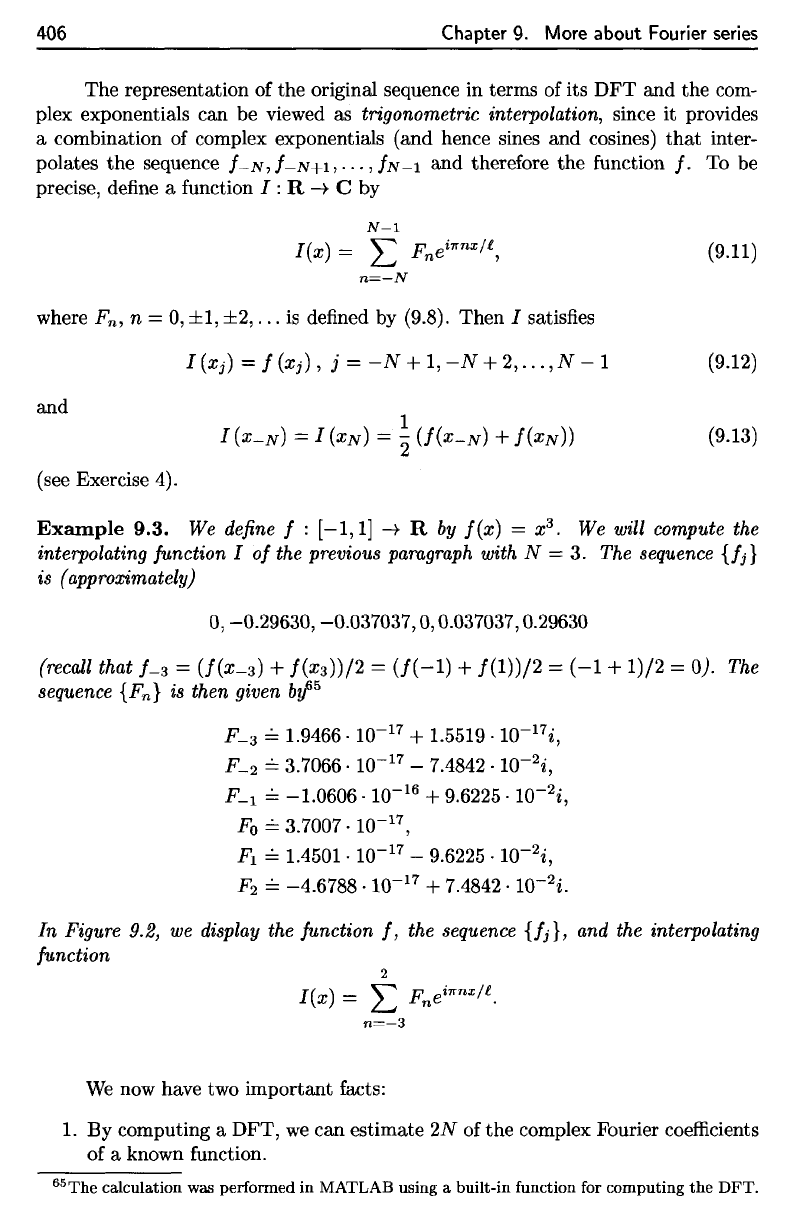
A
simple
formula
for
estimating this integral
is the
so-called (composite) trapezoidal
rule, which replaces
the
integral
by a
discrete
sum
that
can be
interpreted
as the
eiim
rvf
arooc
nf
trar^ovnirlc'
where
h = (b
—
a)/N
and
Xj
= a + jh, j =
0,1,2,...,
N.
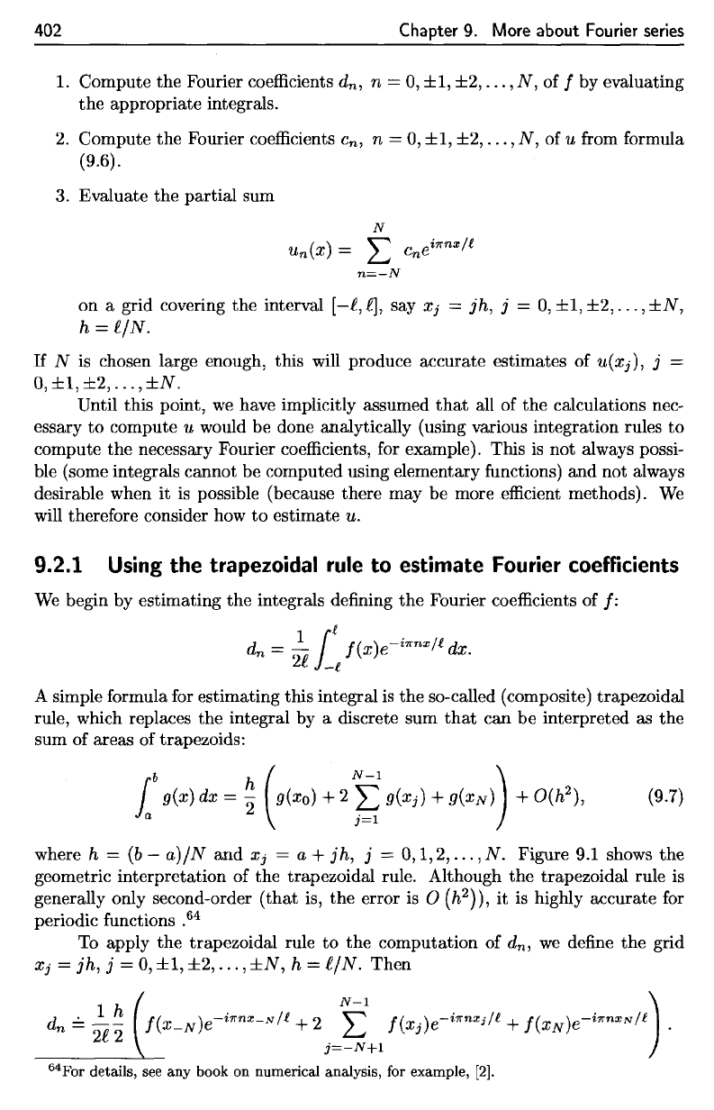
Figure
9.1
shows
the
geometric interpretation
of the
trapezoidal rule. Although
the
trapezoidal rule
is
generally only second-order (that
is, the
error
is O
(h
2
}),
it is
highly accurate
for
periodic
functions
,
64
To
apply
the
trapezoidal rule
to the
computation
of
d
n
,
we
define
the
grid
Xj
=
jh,
j = 0, ±1,
±2,...,
±N, h =
i/N. Then
For
details,
see any
book
on
numerical
analysis,
for
example,
[2].
402
Chapter 9. More about Fourier
series
1. Compute the Fourier coefficients d
n
, n = 0,
±1, ±2,
...
,
N,
of f by evaluating
the
appropriate integrals.
2.
Compute
the
Fourier coefficients en, n = 0,
±1, ±2,
...
,
N,
of u from formula
(9.6).
3. Evaluate
the
partial sum
N
un(x)
= L
cnei7rnx/£
n=-N
on a grid covering
the
interval
[-f,
f], say
Xj
=
jh,
j =
0,
±1,
±2,
...
,
±N,
h =
fiN.
If
N is chosen large enough, this will produce accurate estimates of u(Xj), j =
0,
±1,
±2,
...
,
±N.
Until this point,
we
have implicitly assumed
that
all of
the
calculations nec-
essary
to
compute U would be done analytically (using various integration rules
to
compute
the
necessary Fourier coefficients, for example). This
is
not always possi-
ble (some integrals cannot be computed using elementary functions)
and
not always
desirable when
it
is possible (because there may be more efficient methods).
We
will therefore consider how
to
estimate u.
9.2.1
Using
the trapezoidal
rule
to estimate Fourier coefficients
We
begin by estimating
the
integrals defining
the
Fourier coefficients of
f:
d
n
=
:f
ill
f(x)e-i7rnx/l dx.
A simple formula for estimating this integral
is
the
so-called (composite) trapezoidal
rule, which replaces the integral by a discrete sum
that
can be interpreted as
the
sum of areas of trapezoids:
{b
h (
N-l
)
J
a
g(x) dx
= 2 g(xo) + 2
f;
g(Xj) + g(XN) + O(h2),
(9.7)
where h =
(b
-
a)IN
and
Xj
= a +
jh,
j =
0,1,2,
...
,
N.
Figure 9.1 shows
the
geometric interpretation of the trapezoidal rule. Although
the
trapezoidal rule is
generally only second-order
(that
is,
the
error is 0 (h2)),
it
is highly accurate for
periodic functions
.64
To apply
the
trapezoidal rule
to
the
computation of d
n
,
we
define
the
grid
Xj
=
jh,
j = 0,
±1, ±2,
...
,
±N,
h =
fiN.
Then
d . 1 h
n =
2f2
6
4
For
details, see
any
book
on
numerical analysis, for example,
[2].
9.2. Fourier series
and the FFT
403
Figure
9.1.
Illustration
of the
trapezoidal
rule
for
numerical integration;
the
(signed)
area
under
the
curve
is
estimated
by the
areas
of the
trapezoids.
Since
and
where
and
The
reader should
take
note
of the
special definition
of
f-N,
which reduces
to
simply
f_
N
=
f(x-
N
)
=
/(-£)
when
/ is
2^-periodic
(so
that
f(-l)
=
f(t}}.
The
sequence
of
estimates
F-N,
F_JV+I,
• •
•,
FN-I
is
essentially produced
by
applying
the
discrete Fourier transform
to the
sequence
/-AT,
f-N+i,
• •
•,
/jv-i,
as
we
now
show.
we
can
simplify
this
to
9.2.
Fourier
series
and
the FFT
403
0.2 0.4 0.6 0.8
x
Figure
9.1.
fllustration
of
the trapezoidal rule for numerical integration;
the (signed) area
under
the curve is estimated
by
the areas
of
the trapezoids.
Since
and
h 1 _ i7fnxj _
i7fnj
2f
2N'
l
-]\i'
we
can simplify this
to
N-l
d
..:..
F -
~
'"
f·
-i7rnj/N -
-N -N
ION
- 1
n - n -
~
Je
, n - ,
+,
... , , ... , ,
2N.
N
J=-
(9.8)
where
Ii
=f(xj),
j=-N+l,-N+2,
...
,O,
...
,N-l
and
1
f-N
= 2
(/(-l)
+
f(l)).
The
reader should take note of
the
special definition of f _
N,
which reduces
to
simply
f-N
=
f(X-N)
=
f(-l)
when f
is
21-periodic (so
that
f(-l)
=
f(l)).
The
sequence of estimates
F-N,
F_
N
+1,""
F
N
-
1
is
essentially produced by
applying the
discrete Fourier
transform
to the sequence f - N , f - N +
1,
...
, f N
-1,
as
we
now show.
404
Chapter
9.
More about Fourier
series
9.2.2
The
discrete
Fourier transform
Just
as a
function defined
on
\—i,
—H\
can be
synthesized
from
functions, each having
a
distinct frequency,
so a
finite
sequence
can be
synthesized
from
sequences with
distinct frequencies.
Definition
9.2.
Let
0,0,0,1,...,
OM-I
be a
sequence
of
real
or
complex
numbers.
Then
the
discrete Fourier transform (DFT)
maps
ao,
ai,...,
OM-I
to the
sequence
where
The
original sequence
can be
recovered
by
applying
the
inverse
DFT:
The
proof
of
this relationship
is a
direct calculation
(see
Exercise
5). We
will
often
refer
to the
sequence
A
0
,Ai,...
,AM-I
as the DFT of
ao>«i,
• • •
>«M-I,
although
the
correct
way to
express
the
relationship
is
that
A
0
,Ai,...,
AM-I
is the
image
under
the DFT of
OQ,
ai,...,
OM-I
(the
DFT is the
mapping,
not the
result
of the
mapping). This abuse
of
terminology
is
just
a
convenience,
and is
quite common.
As
another convenience,
we
will
write
the
sequence
00,01,...
,OM-I
as
{aj}
1
^
1
,
or
even just
{a,j}
(if the
limits
of j are
understood).
We
will
now
show
that
the
relationship between
the
sequences
{/jj^T.
1
^
an
d
[Fn}n=-N
can
b
e
expressed
in
terms
of the
DFT. (The
reader
will
recall
that
F
n
=
d
n
,
the nth
Fourier
coefficient
of the
function
/ on
[—I,i}.}
Since
e
lQ
is
27r-periodic,
we
have
We
can
therefore write,
for n =
—N,
—N +
1,...,
N
—
1,
404 Chapter 9. More about Fourier series
9.2.2 The discrete Fourier transform
Just
as a function defined on
[-i,
-f]
can be synthesized from functions, each having
a distinct frequency,
so
a finite sequence can be synthesized from sequences with
distinct frequencies.
Definition
9.2.
Let ao,
al,
...
,
aM
-1
be
a sequence
of
real
or complex numbers.
Then the
discrete Fourier transform
(DFT)
maps
ao,
al,
...
,
aM
-1
to the sequence
where
M-1
A
=
~
"a·e-27rinj/M
n 0 1 M 1
n M
L...J
J ,
=,
,
...
,
-.
j=O
The original sequence can be recovered by applying
the
inverse
DFT:
M-l
. -
"A
27rinj/M . - 0
12M
- 1
a
J
-
L...J
n
e
,
J - , , ,
...
, .
n=O
(9.9)
(9.10)
The proof of this relationship
is
a direct calculation (see Exercise 5).
We
will often
refer
to
the
sequence A
o
,A
1
,
...
,AM-1
as
the
DFT
of
ao,al,
...
,aM-1,
although
the
correct way
to
express
the
relationship
is
that
A
o
, A
1
,
...
,
AM
-1
is the image
under the
DFT
of ao, a1,
...
,
aM-l
(the
DFT
is
the mapping, not the result of the
mapping). This abuse of terminology is just a convenience, and
is
quite common.
As
another convenience,
we
will write the sequence ao, a1,
...
,
aM
-1
as
{aj}
~01,
or even
just
{aj}
(if
the limits of j are understood).
We
will now show
that
the relationship between the sequences {fJ
}.f=--.!-N
and
{Fn};;==-~N
can be expressed in terms of
the
DFT. (The reader will recall
that
Fn
==
d
n
,
the
nth
Fourier coefficient of
the
function f on
[-i,i].)
Since e
i
()
is
27r-periodic,
we
have
e-7ri(j+2N)n/N =
e-7rijn/N-27rin
=
e-7rijn/N
e-
27rin
= e-7rijn/N.
We
can therefore write, for n =
-N,
-N
+
1,
...
, N -
1,
9.2. Fourier
series
and the FFT
405
If
we
define
a
sequence
{fj}?=
0
*
^
then
we
have
Moreover,
by the
periodicity
of
e
ze
,
we can
write
Defining
the
sequence
(F
n
}^
0
l
by
we
have
Thus
{F
n
}
is the DFT of
{/j}.
With
this
rearrangement
of
terms understood,
we
can say
that
{F
n
}
is the DFT of
{fj}.
To
actually compute
{F
n
}n=-N
f
rom
{/jljL^-V'
we
perform
the
following
three steps:
1.
Replace
the
sequence
with
and
label
the
latter sequence
as
{fj}
2
j~
0
l
.
2.
Compute
the DFT of
{fj}
2
^
1
to get
{F
n
}^-i.
3.
The
desired sequence
{F
n
}^~^
N
is
9.2. Fourier
series
and
the FFT
=
2~
L
/je-1rijn/N
+ L
/j_2Ne-1rijn/N
.
{
N-l
2N-l
}
j=O
j=N
If
we
define a sequence
{jj}~:O-1
by
J.
= {
Ij,
j=0,1,
...
,N-1,
)
/j-2N,
j = N, N + 1,
...
,
2N
- 1,
then
we
have
2N-l
F
-
1
"1-
-1rijn/N
- N N + 1 N 1
n -
2N
~
je
, n - - , - ,
...
,
-.
)=0
Moreover, by the periodicity of e
ifJ
,
we
can write
2N-l
F =
~
"
1-·e-
1rij
(n+2N)/N
N
NIl
n
2N
~
J , n = - , - + , ... , - .
j=O
n = O,l,
...
,N
-
1,
n = N, N +
1,
...
,
2N
-
1,
we
have
2N-l
F:
=
_1_
"
f-·e-1rijn/N
0 1
2N
1
n
2N
~
J , n = , ,
...
,
-.
j=O
405
Thus {Fn}
is
the
DFT
of
{]j}. With this rearrangement of terms understood,
we
can say
that
{Fn}
is
the
DFT
ofJ/j}.
To actually compute
{Fn}n~~N
from
{fj}f=-lN'
we
perform
the
following
three steps:
1. Replace the sequence
!-N'···'
1-1,
to,
It,···,
IN-l
with
10,
It,···,
!N-I,
I-N'
...
'
1-1,
and label
the
latter sequence as
{]j}
~:0-1
.
-
2N-l
-
2N-l
2.
Compute
the
DFT
of
{!j}j=o
to
get
{Fn}n=O
.
3.
The
desired sequence
{Fn};;==-~N
is
(see
Exercise
4).
We
now
have
two
important facts:
1.
By
computing
a
DFT,
we can
estimate
IN
of the
complex Fourier
coefficients
of
a
known function.
65
The
calculation
was
performed
in
MATLAB using
a
built-in
function
for
computing
the
DFT.
406
Chapter
9.
More
about
Fourier
series
The
representation
of the
original sequence
in
terms
of its DFT and the
com-
plex exponentials
can be
viewed
as
trigonometric interpolation, since
it
provides
a
combination
of
complex exponentials (and hence sines
and
cosines)
that
inter-
polates
the
sequence
/_AT,/_JV+I,-•
•
,/JY-I
and
therefore
the
function
/. To be
precise,
define
a
function
/ : R
-»
C by
where
F
n
,
n = 0, ±1,
±2,...
is
defined
by
(9.8).
Then
/
satisfies
and
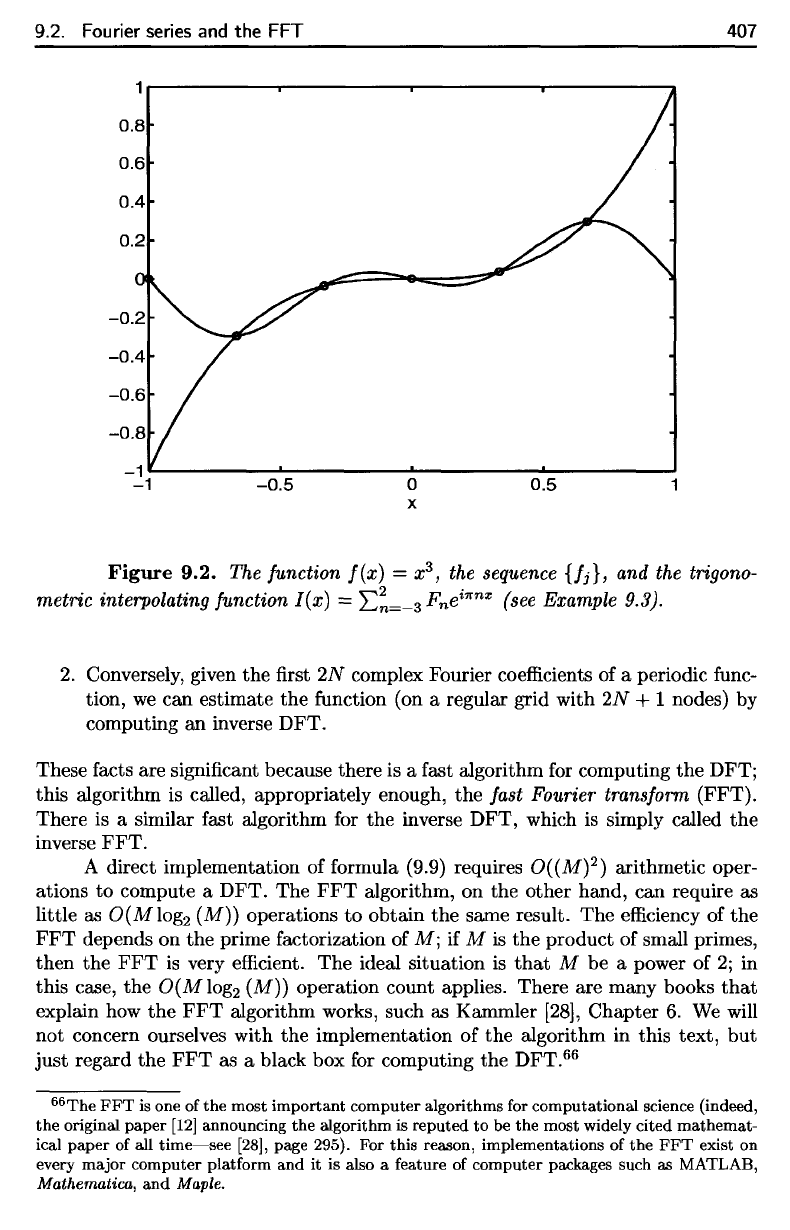
Example
9.3.
We
define
f
:
[—1,1]
—>•
R by
/(#)
=
x
3
.
We
will
compute
the
interpolating
function
I
of
the
previous
paragraph
with
N = 3. The
sequence
{fj}
is
(approximately)
(recall
that
/_
3
-
(f(x-
3
)
+
fM)/2
=
(/(-I)
+
/(l))/2
= (-1 +
l)/2
=
Q).
The
sequence
{F
n
}
is
then given
by
65
In
Figure 9.2,
we
display
the
function
f,
the
sequence
{fj},
and the
interpolating
function
406
Chapter
9.
More about Fourier
series
The
representation of
the
original sequence in terms of its
DFT
and
the
com-
plex exponentials can be viewed as
trigonometric interpolation, since
it
provides
a combination of complex exponentials (and hence sines
and
cosines)
that
inter-
polates
the
sequence f
-N
, f
-N
+
1,
...
, fN
-1
and
therefore
the
function
f.
To be
precise, define a function
I : R
--t
C by
N-1
I(x) = L
(9.11)
n=-N
where Fn, n =
0,
±1, ±2,
...
is
defined by (9.8). Then I satisfies
I
(Xj)
= 1 (Xj) , j = -N +
1,
- N +
2,
...
,N
- 1
(9.12)
and
(9.13)
(see Exercise 4).
Example
9.3.
We define f :
[-1,1]
--t
R
by
f(x)
=
X3.
We will compute the
interpolating function I
of
the previous paragraph with N = 3. The sequence
{h}
is (approximately)
0,
-0.29630, -0.037037,0,0.037037,0.29630
(recall that
1-3
= (f(X-3) + f(X3))/2 =
(f(-1)
+ f(1))/2 =
(-1
+
1)/2
= 0). The
sequence {Fn}
is
then given by
65
F_
3
==
1.9466.10-
17
+ 1.5519. 1O-
17
i,
F-2
==
3.7066.10-
17
- 7.4842· 1O-
2
i,
F-1
==
-1.0606.10-
16
+ 9.6225· 1O-
2
i,
Fo
==
3.7007.10-
17
,
Fl
==
1.4501·
10-
17
- 9.6225· 1O-
2
i,
F2
==
-4.6788.10-
17
+ 7.4842· 1O-
2
i.
In Figure 9.2,
we
display the function f, the sequence
{h},
and the interpolating
function
2
I(x) = L Fnei7rnx/l.
n=-3
We
now have two
important
facts:
1. By computing a
DFT,
we
can estimate
2N
of
the
complex Fourier coefficients
of
a known function.
65The
calculation
was
performed
in
MATLAB
using a
built-in
function for
computing
the
DFT.
9.2.
Fourier
series
and the FFT
407
Figure
9.2.
The
function
f(x)
—
x
3
,
the
sequence
{fj},
and the
trigono-
metric
interpolating
function
I(x)
=
X)
n
__
3
F
n
e
twnx
(see
Example
9.3).
2.
Conversely, given
the first
2AT
complex Fourier
coefficients
of a
periodic
func-
tion,
we can
estimate
the
function
(on a
regular grid with
IN
+ 1
nodes)
by
computing
an
inverse DFT.
These facts
are
significant because there
is a
fast algorithm
for
computing
the
DFT;
this
algorithm
is
called, appropriately enough,
the
fast
Fourier
transform
(FFT).
There
is a
similar fast algorithm
for the
inverse DFT, which
is
simply called
the
inverse
FFT.
A
direct implementation
of
formula (9.9) requires
O((M)
2
)
arithmetic oper-
ations
to
compute
a
DFT.
The FFT
algorithm,
on the
other hand,
can
require
as
little
as
O(Mlog
2
(M))
operations
to
obtain
the
same result.
The
efficiency
of the
FFT
depends
on the
prime factorization
of
M;
if
M
is the
product
of
small primes,
then
the FFT is
very
efficient.
The
ideal situation
is
that
M be a
power
of 2; in
this case,
the
O(Mlog
2
(M))
operation count applies. There
are
many books
that
explain
how the FFT
algorithm works, such
as
Kammler
[28], Chapter
6. We
will
not
concern ourselves with
the
implementation
of the
algorithm
in
this
text,
but
just regard
the FFT as a
black
box for
computing
the
DFT.
66
66
The
FFT is one of the
most important computer algorithms
for
computational science (indeed,
the
original paper [12] announcing
the
algorithm
is
reputed
to be the
most widely cited mathemat-
ical
paper
of all
time—see
[28], page 295).
For
this reason, implementations
of the FFT
exist
on
every
major computer platform
and it is
also
a
feature
of
computer packages such
as
MATLAB,
Mathematica^
and
Maple.
9.2. Fourier series and
the
FFT
0.8
0.6
0.4
0.2
o
x
0.5
407
Figure
9.2.
The function
f(x)
= x
3
,
the sequence
{Ii},
and the trigono-
metric interpolating function
lex)
=
L~=-3
Fnei1rnx (see Example 9.3).
2. Conversely, given
the
first
2N
complex Fourier coefficients of a periodic func-
tion,
we
can estimate
the
function (on a regular grid with
2N
+ 1 nodes) by
computing
an
inverse
DFT.
These facts are significant because there is a fast algorithm for computing
the
DFT;
this algorithm is called, appropriately enough,
the
fast Fourier transform
(FFT).
There is a similar fast algorithm for
the
inverse
DFT,
which is simply called
the
inverse
FFT.
A direct implementation of formula (9.9) requires O((M)2) arithmetic oper-
ations
to
compute a
DFT.
The
FFT
algorithm, on the
other
hand, can require as
little as
OeM
log2
(M)) operations
to
obtain
the
same result.
The
efficiency of
the
FFT
depends on
the
prime factorization of
M;
if M is
the
product of small primes,
then
the
FFT
is
very efficient.
The
ideal situation is
that
M
be
a power of 2; in
this case,
the
OeM
log2
(M)) operation count applies. There are many books
that
explain how
the
FFT
algorithm works, such as Kammler
[28],
Chapter
6.
We
will
not concern ourselves with
the
implementation
of
the
algorithm in this
text,
but
just
regard
the
FFT
as a black box for computing
the
DFT.66
66The
FFT
is one of
the
most
important
computer
algorithms for
computational
science (indeed,
the
original
paper
[12]
announcing
the
algorithm
is
reputed
to
be
the
most
widely cited
mathemat-
ical
paper
of all
time-see
[28],
page 295). For this reason,
implementations
of
the
FFT
exist
on
every
major
computer
platform
and
it
is also a feature of
computer
packages such as MATLAB,
Mathematica,
and
Maple.