Gockenbach M.S. Partial Differential Equations. Analytical and Numerical Methods
Подождите немного. Документ загружается.

378
Chapter
8.
Problems
in
multiple
spatial dimensions
The
last step
follows
from
the
fact
that
v
vanishes
on
dtl.
We
define
the
bilinear
form
a(-,
•) by
We
then obtain
the
weak
form
of the BVP
(8.52):
The
proof
that
a
solution
of the
weak
form
also
satisfies
the
original
BVP
follows
the
same
pattern
as in
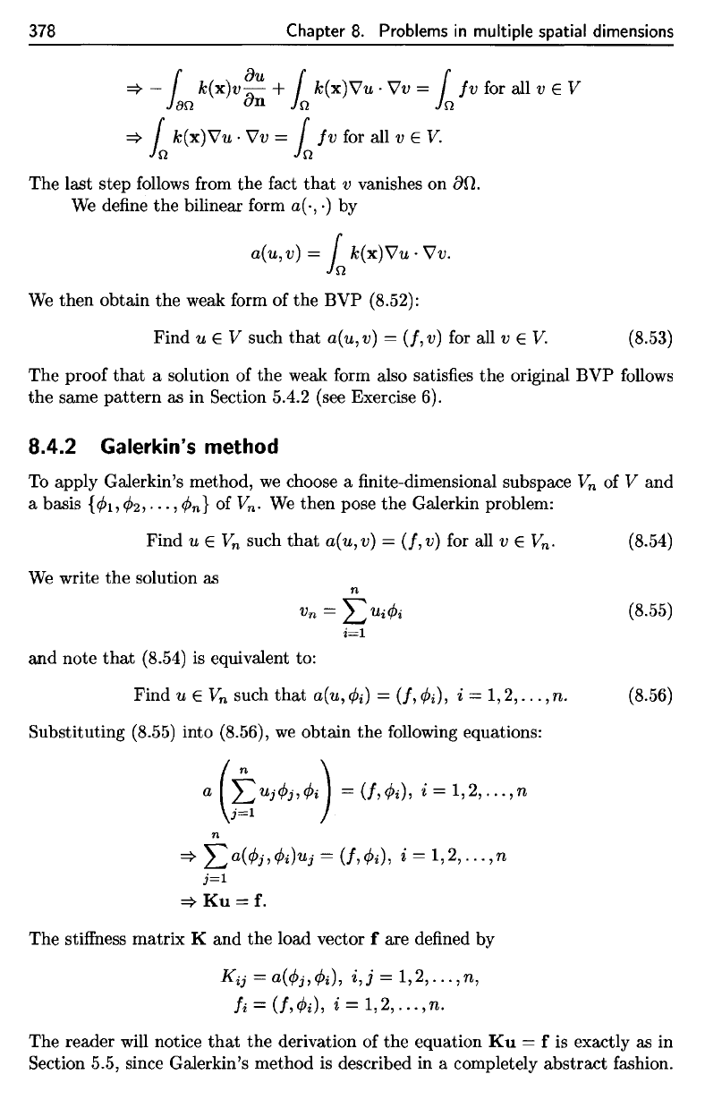
Section 5.4.2 (see Exercise
6).
8.4.2
Galerkin's
method
To
apply Galerkin's method,
we
choose
a finite-dimensional
subspace
V
n
of V and
a
basis
{^1,^2,
• •
•,
<f>
n
}
ofV
n
.
We
then pose
the
Galerkin
problem:
We
write
the
solution
as
and
note
that
(8.54)
is
equivalent
to:
Substituting (8.55) into (8.56),
we
obtain
the
following
equations:
The
stiffness
matrix
K and the
load vector
f are
defined
by
The
reader
will
notice
that
the
derivation
of the
equation
Ku
=
f is
exactly
as in
Section 5.5, since Galerkin's method
is
described
in a
completely
abstract
fashion.
378
Chapter
8.
Problems
in
multiple spatial dimensions
=>
- {
k(x)v
~u
+ {
k(x)\7u·
\7v = (
Jv
for all v E V
ien
un
in in
=>
In
k(x)\7u
. \7v =
In
Jv
for all v E
V.
The last step follows from the fact
that
v vanishes on
an.
We
define
the
bilinear form a(·,
.)
by
a(u,v)
=
In
k(x)\7u·
\7v.
We
then obtain the weak form of the
BVP
(8.52):
Find
u E V such
that
a(
u,
v) =
(f,
v) for all v E
V.
(8.53)
The
proof
that
a solution of the weak form also satisfies
the
original
BVP
follows
the
same
pattern
as in Section 5.4.2 (see Exercise 6).
8.4.2 Galerkin's method
To
apply Galerkin's method,
we
choose a finite-dimensional subspace
Vn
of V and
a basis
{(1)1,
¢2,···,
¢n}
of V
n
·
We
then pose
the
Galerkin problem:
Find
u E
Vn
such
that
a(u,v)
=
(f,v)
for all v E V
n
. (8.54)
We
write the solution as
n
Vn
=
LUi¢i
i=1
and
note
that
(8.54)
is
equivalent to:
(8.55)
Find
U E
Vn
such
that
a(
u,
¢i) =
(f,
¢i), i = 1,2,
...
,
n.
(8.56)
Substituting (8.55) into (8.56),
we
obtain
the
following equations:
n
=>
La(¢j,¢i)Uj
=
(f,¢i),
i =
1,2,
...
,n
j=1
=>
Ku
= f.
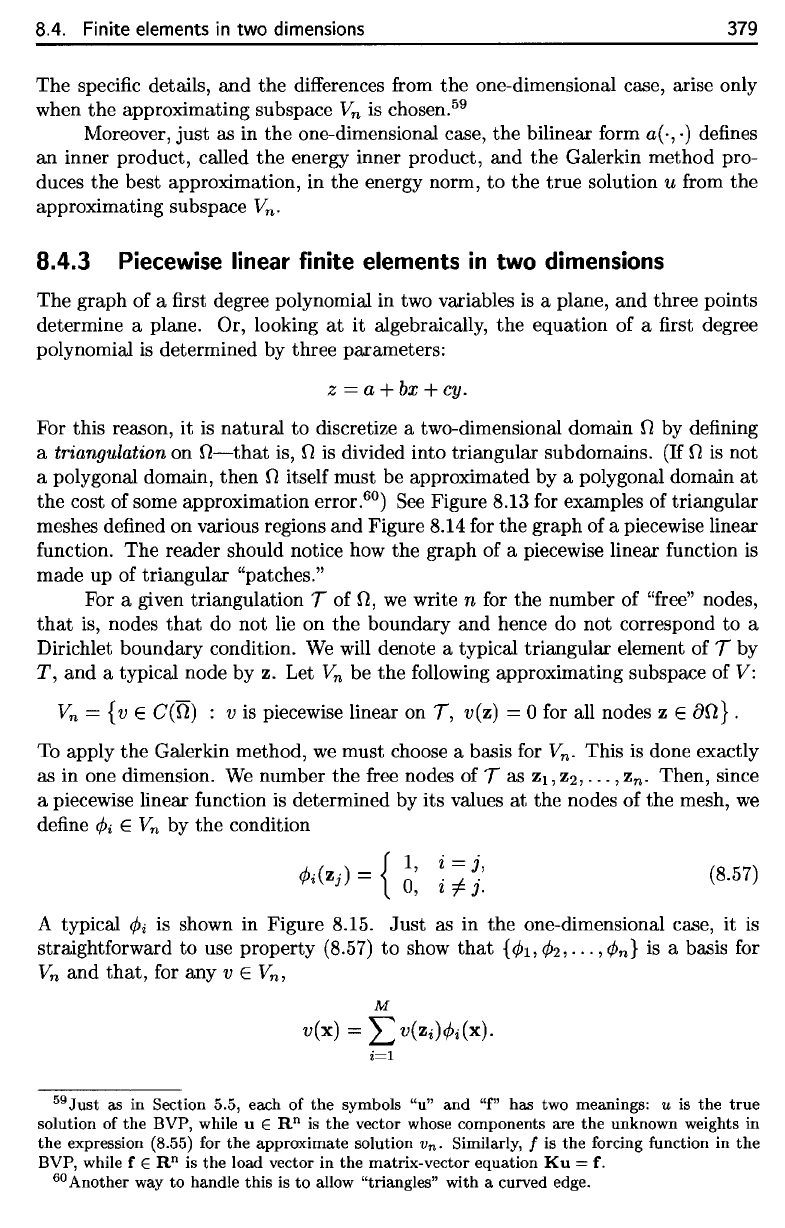
The stiffness matrix K and the load vector f are defined by
Kij = a(¢j,¢i),
i,j
=
1,2,
...
,n,
Ji
=
(f,¢i),
i = 1,2,
...
,no
The reader will notice
that
the
derivation of the equation
Ku
= f is exactly as in
Section 5.5, since Galerkin's method
is
described in a completely abstract fashion.
59
Just
as in
Section 5.5, each
of the
symbols
"u"
and
"f"
has two
meanings:
u is the
true
solution
of the
BVP,
while
u
G
R
n
is the
vector whose components
are the
unknown
weights
in
the
expression (8.55)
for the
approximate solution
v
n
.
Similarly,
/ is the
forcing
function
in the
BVP,
while
f
e
R
n
is the
load vector
in the
matrix-vector
equation
Ku =
f.
60
Another
way to
handle this
is to
allow "triangles" with
a
curved edge.
8.4.
Finite
elements
in two
dimensions
379
The
specific
details,
and the
differences
from
the
one-dimensional case, arise only
when
the
approximating
subspace
V
n
is
chosen.
59
Moreover,
just
as in the
one-dimensional
case,
the
bilinear
form
a(-,
•)
defines
an
inner product, called
the
energy inner product,
and the
Galerkin method pro-
duces
the
best approximation,
in the
energy norm,
to the
true solution
u
from
the
approximating subspace
V
n
.
8.4.3 Piecewise linear finite elements
in two
dimensions
The
graph
of a first
degree polynomial
in two
variables
is a
plane,
and
three points
determine
a
plane.
Or,
looking
at it
algebraically,
the
equation
of a first
degree
polynomial
is
determined
by
three parameters:
For
this reason,
it is
natural
to
discretize
a
two-dimensional domain
fU
by
defining
a
triangulation
on
fi—that
is,
f)
is
divided into triangular subdomains.
(If
il
is not
a
polygonal domain, then
f)
itself must
be
approximated
by a
polygonal domain
at
the
cost
of
some approximation
error.
60
)
See
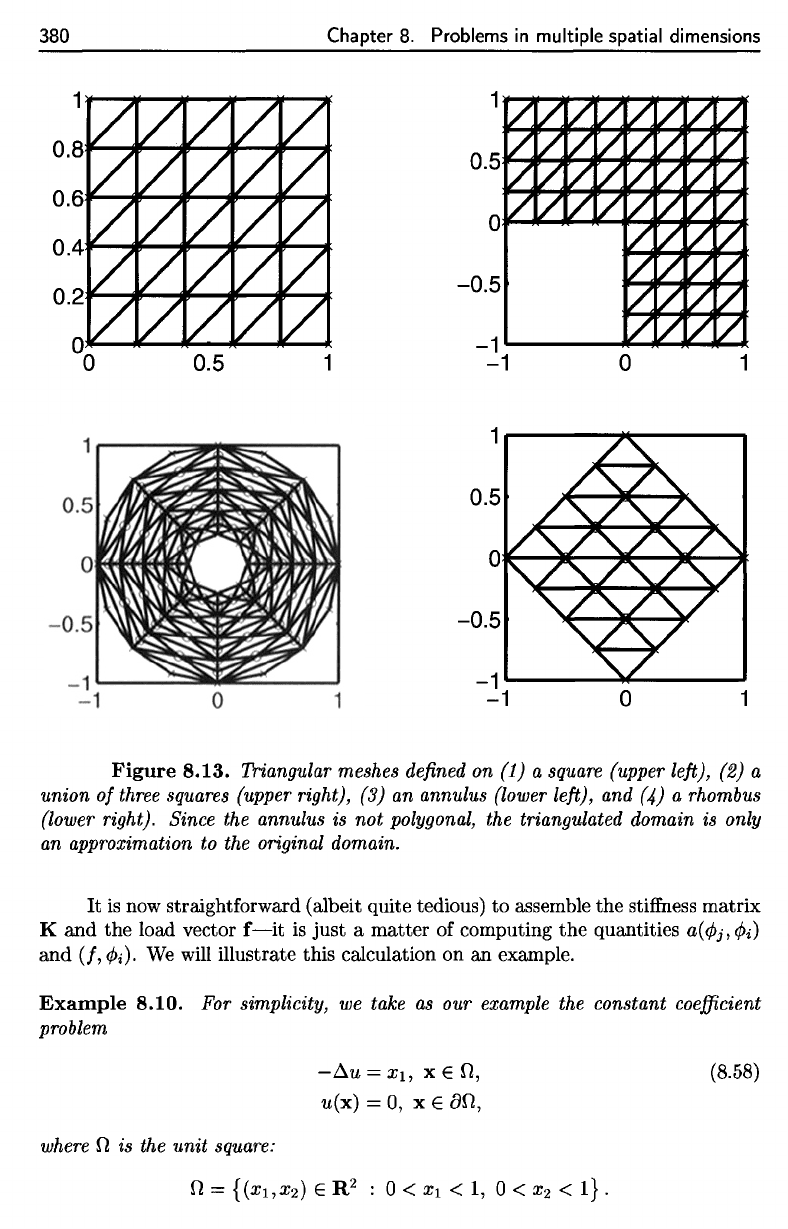
Figure 8.13
for
examples
of
triangular
meshes
defined
on
various regions
and
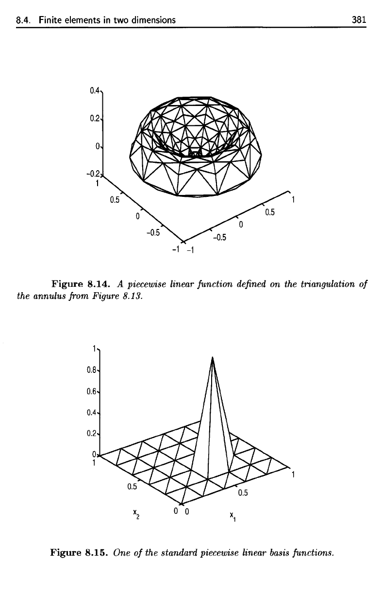
Figure
8.14
for the
graph
of a
piecewise linear
function.
The
reader should notice
how the
graph
of a
piecewise linear
function
is
made
up of
triangular
"patches."
For
a
given triangulation
T of
il,
we
write
n
for the
number
of
"free"
nodes,
that
is,
nodes
that
do not lie on the
boundary
and
hence
do not
correspond
to a
Dirichlet boundary condition.
We
will
denote
a
typical triangular element
of T by
T, and a
typical node
by z. Let
V
n
be the
following
approximating subspace
of
V:
V
n
= {v €
C(fi)
: v is
piecewise linear
on T,
v(z)
= 0 for all
nodes
z 6
dfl}
.
To
apply
the
Galerkin method,
we
must choose
a
basis
for
V
n
.
This
is
done exactly
as in one
dimension.
We
number
the
free
nodes
of T as
z
i5
z
2
,...,z
n
.
Then, since
a
piecewise linear
function
is
determined
by its
values
at the
nodes
of the
mesh,
we
define
fa
e
V
n
by the
condition
A
typical
<fo
is
shown
in
Figure 8.15.
Just
as in the
one-dimensional
case,
it is
straightforward
to use
property (8.57)
to
show
that
{</>i,
02,
• •
•,
0n}
is a
basis
for
V
n
and
that,
for any v 6
V
n
,
8.4. Finite elements in
two
dimensions
379
The
specific details,
and
the
differences from
the
one-dimensional case, arise only
when
the
approximating subspace
Vn
is chosen.
59
Moreover,
just
as in
the
one-dimensional case,
the
bilinear form a(·,·) defines
an inner product, called
the
energy inner product,
and
the
Galerkin method pro-
duces
the
best approximation, in
the
energy norm,
to
the
true
solution u from
the
approximating subspace V
n
.
8.4.3 Piecewise linear finite elements
in
two
dimensions
The
graph of a first degree polynomial in two variables
is
a plane,
and
three points
determine a plane. Or, looking
at
it algebraically,
the
equation of a first degree
polynomial is determined by three parameters:
z =
a+bx+cy.
For this reason,
it
is
natural
to
discretize a two-dimensional domain 0 by defining
a
triangulation on
O-that
is, 0 is divided into triangular subdomains. (If 0 is
not
a polygonal domain,
then
0 itself must be approximated by a polygonal domain
at
the
cost of some approximation error. 60)
See
Figure 8.13 for examples of triangular
meshes defined on various regions
and
Figure 8.14 for
the
graph of a piecewise linear
function.
The
reader should notice how
the
graph of a piecewise linear function is
made up of triangular "patches."
For a given triangulation 7 of
0,
we
write n for
the
number of "free" nodes,
that
is, nodes
that
do not lie on
the
boundary
and
hence do not correspond
to
a
Dirichlet boundary condition.
We
will denote a typical triangular element of 7 by
T,
and
a typical node by z. Let
Vn
be
the
following approximating subspace of V:
Vn
=
{v
E C(O) : v
is
piecewise linear on
7,
v(z) = 0 for all nodes z E
aO}
.
To apply
the
Galerkin method,
we
must choose a basis for V
n
.
This
is
done exactly
as in one dimension.
We
number
the
free nodes of 7 as
Z1, Z2,
...
,
Zn.
Then, since
a piecewise linear function
is
determined by its values
at
the nodes
of
the
mesh,
we
define
~i
E
Vn
by
the
condition
,j,
()
{I,
i =
j,
'l'i
Zj
= 0 .
...t..
, Z I
J.
(8.57)
A typical
~i
is shown in Figure 8.15.
Just
as in
the
one-dimensional case,
it
is
straightforward
to
use property
(8.57)
to
show
that
{~1'
~2'
...
'
~n}
is a basis for
Vn
and
that,
for any v E V
n
,
M
v(x) =
2.:
V(Zi)~i(X).
i=1
59
Just
as in Section 5.5, each of
the
symbols "u"
and
"f" has two meanings: u is
the
true
solution of
the
BVP, while u E
Rn
is
the
vector whose components are the unknown weights in
the
expression (8.55) for
the
approximate solution
Vn.
Similarly, f is
the
forcing function in
the
BVP, while
fERn
is
the
load vector in
the
matrix-vector equation
Ku
=
f.
60
Another
way
to
handle
this
is
to
allow "triangles" with a curved edge.
380
Chapter
8.
Problems
in
multiple spatial dimensions
Figure
8.13. Triangular meshes
defined
on (1) a
square
(upper
left),
(2) a
union
of
three squares
(upper
right),
(3) an
annulus (lower
left),
and (4) a
rhombus
(lower
right). Since
the
annulus
is not
polygonal,
the
triangulated domain
is
only
an
approximation
to the
original domain.
It is now
straightforward
(albeit
quite
tedious)
to
assemble
the
stiffness
matrix
K and the
load
vector
f—it
is
just
a
matter
of
computing
the
quantities
o(0j,0f)
and
(/,<&).
We
will
illustrate
this
calculation
on an
example.
Example
8.10.
For
simplicity,
we
take
as our
example
the
constant
coefficient
problem
where
£)
is the
unit
square:
380
Chapter
8.
Problems
in
multiple spatial dimensions
-0.5
-1~----~~~~~
-1
o
1
1
1r-----~~----~
0.5
0.5
0
- 0.5
-0.5
- 1
-1~----~~-----J
- 1
0
1
-1
o
1
Figure
8.13.
Triangular meshes defined on (1) a square (upper left), (2) a
union
of
three squares (upper right), (3) an annulus (lower left), and (4) a rhombus
(lower right). Since the annulus is
not
polygonal, the triangulated domain is only
an approximation to the original domain.
It
is
now straightforward (albeit quite tedious) to assemble the stiffness matrix
K
and
the
load vector
f-it
is
just
a
matter
of computing
the
quantities
a(
<Pj,
<Pi)
and
(J,
<Pi).
We
will illustrate this calculation on
an
example.
Example
8.10.
For simplicity, we take
as
our example the constant coefficient
problem
where
n is the unit square:
-~U=Xl,
xEn,
u(x)
=
0,
x E
an,
(8.58)
8.4. Finite elements
in two
dimensions
381
Figure 8.14.
A
piecewise linear function
defined
on the
triangulation
of
the
annulus
from
Figure
8.13.
Figure
8.15.
One of the
standard piecewise linear basis
functions.
8.4. Finite elements
in
two dimensions
0.4
0.2
o
-0.2
1
-1 -1
381
Figure
8.14.
A piecewise linear function defined on the triangulation
of
the annulus from Figure 8.13.
o 0
Figure
8.15.
One
of
the standard piecewise linear basis functions.
382
Chapter
8.
Problems
in
multiple
spatial
dimensions
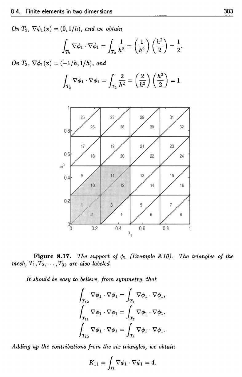
We
choose
a
regular
triangulation
with
32
triangles,
25
nodes,
and 9
free
nodes.
The
mesh
is
shown
in
Figure 8.16, with
the
free
nodes
labeled
from
1 to 9.
61
As we
explained
in
Section 5.6,
the
support
of a
function
is the set on
which
the
function
is
nonzero, together with
the
boundary
of
that
set.
Figure
8.16.
The
mesh
for
Example 8.10.
We
begin
with
the
computation
of
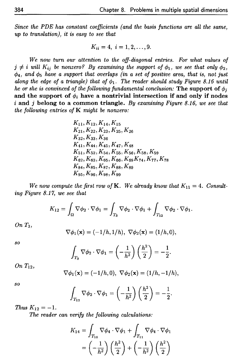
The
support?
1
of fa is
shown
in
Figure 8.17, which
also
labels
the
triangles
in the
mesh,
TI
,
TI
,...,
Ts2.
This support
is
made
up of six
triangles;
on
each
of
these
triangles,
fa has a
different
formula.
We
therefore
compute
KH
by
adding
up the
contributions from
each
of the six
triangles:
On
TI,
V0i(x)
=
(l//i,
0),
where
h
= 1/4
(observing
how fa
changes
along
the
horizontal
and
vertical
edges
ofTi
leads
to
this conclusion).
The
area
ofTi
(and
of
all the
other triangles
in the
mesh)
is
/i
2
/2.
Thus,
382
Chapter
8.
Problems
in
multiple spatial dimensions
We choose a regular triangulation with
32
triangles, 25 nodes, and 9 free nodes.
The mesh is shown
in
Figure 8.16, with the free nodes labeled from 1 to
9.
Figure
8.16.
The mesh for Example 8.10.
We begin with the computation
of
K11
=
a((/h,¢>d
= k \l¢>l' \l¢>l'
The support!H
of
¢>l
is shown
in
Figure 8.17, which also labels the triangles
in
the
mesh, T
1
,
T
2
,
•..
, T
32
• This support is made up
of
six triangles; on each
of
these
triangles,
¢>l
has a different formula. We therefore compute
K11
by adding up the
contributions from each
of
the six triangles;
r
\l¢>l
.
\l¢>l
= r \l¢>l'
\l¢>l
+ r \l¢>l'
\l¢>l
+ r \l¢>l'
\l¢>l
k
in
h h
+ r
\l
¢>l
.
\l
¢>l
+ r
\l
¢>l
.
\l
¢>l
+ r
\l
¢>l
.
\l
¢>l
.
~o
i
nl
in2
On T
1
,
\l¢>l(X)
= (l/h,O), where h =
1/4
(observing how
¢>l
changes along
the horizontal and vertical edges
ofT
1
leads to this conclusion). The
area
ofT
1
(and
of
all the other triangles
in
the mesh) is h
2
/2. Thus,
hi
\l
¢>l
.
\l
¢>l
=
hi
:2
=
(:2)
(~2)
=
~.
61 As
we
explained in Section 5.6,
the
support
of a function is
the
set
on
which
the
function is
nonzero,
together
with
the
boundary
of
that
set.
8.4.
Finite elements
in two
dimensions
383
On
T-2,
V^i(x)
= (0,
l/h),
and we
obtain
On
T
3
,
V^i(x)
=
(-1/fc,
l/h),
and
Figure
8.17.
The
support
of
4>i
(Example
8.10).
The
triangles
of the
mesh,
TI
,
T-2,...,
T
32
are
also
labeled.
It
should
be
easy
to
believe, from
symmetry,
that
Adding
up the
contributions from
the six
triangles,
we
obtain
8.4. Finite elements
in
two dimensions 383
On T
2
,
V'4>1(X)
= (0,
I/h),
and
we
obtain
On T
3
,
V'4>1(X)
=
(-l/h,
I/h),
and
Figure
8.17.
The support
of
4>1
(Example 8.10). The triangles
of
the
mesh, T
1
,
T
2
,
•.•
,T
32
are
also
labeled.
It
should
be
easy to believe, from symmetry, that
Adding up the contributions from the six triangles,
we
obtain
Kll
= k
V'4>1
.
V'4>1
= 4.
384
Chapter
8.
Problems
in
multiple
spatial dimensions
Since
the PDE has
constant
coefficients
(and
the
basis
functions
are all the
same
up
to
translation),
it is
easy
to see
that
We
now
turn
our
attention
to the
off-diagonal
entries.
For
what values
of
j
^
i
will
Kij
be
nonzero
? By
examining
the
support
of fa, we see
that
only
fa,
04,
and 05
have
a
support
that
overlaps
(in a set
of
positive
area,
that
is, not
just
along
the
edge
of a
triangle) that
of fa. The
reader
should study Figure
8.16
until
he
or she is
convinced
of
the
following fundamental conclusion:
The
support
of fa
and the
support
of fa
have
a
nontrivial intersection
if and
only
if
nodes
i
and j
belong
to a
common triangle.
By
examining Figure
8.16,
we see
that
the
following entries
of
K
might
be
nonzero:
We
now
compute
the first row
ofK.
We
already
know that
KH
= 4.
Consult-
ing
Fiaure
8.17,
we see
that
OnT
3
,
so
On
T
12
,
so
Thus
Ki2
= -l.
The
reader
can
verify
the
following calculations:
384
Chapter
8.
Problems
in
multiple spatial dimensions
Since the
PDE
has constant coefficients (and the basis functions
are
all
the same,
up
to translation),
it
is easy to see that
Kii
=
4,
i = 1,2,
...
,9.
We
now turn our attention to the off-diagonal entries. For what values
of
j
=I-
i will
Kij
be
nonzero?
By
examining the support
of
(PI,
we
see that only
<P2,
<P4,
and
<P5
have a support that overlaps (in a set
of
positive
area,
that is, not just
along the
edge
of
a triangle) that
of
<Pl.
The reader should study Figure 8.16 until
he or she
is convinced
of
the following fundamental conclusion:
The
support
of
<Pj
and
the
support
of
<Pi
have
a
nontrivial
intersection
if
and
only
if
nodes
i
and
j
belong
to
a
common
triangle.
By
examining Figure 8.16,
we
see that
the following entries
of
K might
be
nonzero:
Ku,
K
12
, K
14
, K
15
K
21
, K
22
, K
23
,
K
25
, K
26
K32,K33,K36
K41,
K
44
, K
45
, K
47
,
K48
K51,
K
52
, K
54
, K
55
, K
56
, K
58
,
K59
K
62
, K
63
, K
65
, K
66
, K
69
K
74
, K
77
,
K78
K
84
, K
85
, K
87
, K
88
,
K89
K95,K96,K98,K99
We now compute the first row
of
K.
We already know that
Kll
= 4. Consult-
ing Figure
8.17,
we
see that
\7
<Pi
(x) =
(-llh,
Ilh),
\7<P2(X)
= (1Ih,o),
so
On
T
12
,
\7<pl(X)
=
(-llh,
0),
\7<p2(X)
= (1Ih,
-llh),
so
Thus
K12
=
-1.
The reader can verify the following calculations:
8.4.
Finite
elements
in two
dimensions
385
The
rest
of
the
calculations
are
similar,
and the
result
is the
following
stiffness
matrix:
which
is
quite tedious when done
by
hand (unlike
V0j,
0j
itself
is not
piecewise
constant).
We
just
show
one
representative calculation.
We
have
To
compute
the
load
vector
f,
we
must
evaluate
the
integrals
Therefore,
8.4.
Finite
elements
in
two
dimensions
385
=
-1,
K
15
= 1
\l¢5'
\l¢l
+ 1
\l¢5'
\l¢l
Tn
T12
=
(0)
(~2)
+
(0)
(h;)
=0.
The rest
of
the calculations
are
similar, and the result is the following stiffness
matrix:
4
-1
0
-1
0
0 0 0 0
-1
4
-1
0
-1
0 0 0 0
0
-1
4
0 0
-1
0 0 0
-1
0 0 4
-1
0
-1
0 0
K=
0
-1
0
-1
4
-1
0
-1
0
0 0
-1
0
-1
4
0
0
-1
0 0 0
-1
0 0
4
-1
0
0 0 0 0
-1
0
-1
4
-1
0 0 0
0 0
-1
0
-1
4
To
compute the
load
vector f,
we
must
evaluate the integrals
L f(x)¢i(X)
dx,
which is quite tedious when done
by
hand (unlike
\l¢i,
¢i itself is not piecewise
constant). We
just
show one representative calculation. We have
Xl
X E T
1
,
h'
X2
X E T
2
,
h'
X2-X1+h
X E T
3
,
h
,
¢1(Xl,X2) =
Xl-X2+h
X E T
lO
,
h
,
2h-X2
X E T
u
,
-h-
,
2h-X1
X E T
12
,
-h-
,
0,
otherwise.
Therefore,
386
Chapter
8.
Problems
in
multiple
spatial dimensions
Continuing
in
this manner,
we find
We
can now
solve
62
Ku = f to
obtain
The
resulting piecewise linear approximation
is
displayed
in
Figure
8.18.
The
calculations
in the
previous example
are
elementary,
but
extremely time-
consuming,
and are
ideal
for
implementation
in a
computer program. When these
calculations
are
programmed,
the
operations
are not
organized
in the
same
way as
in
the
above hand calculation.
For
example, instead
of
computing
one
entry
in K
at a
time,
it is
common
to
loop over
the
elements
of the
mesh
and to
compute
all
the
contributions
to the
various
entries
in K and f
from
each element
in
turn.
Among
other things, this
simplifies
the
data
structure
for
describing
the
mesh.
(To
automate
the
calculations presented above,
it
would
be
necessary
to
know, given
a
certain node, which nodes
are
adjacent
to it.
This
is
avoided when
one
loops over
the
elements instead
of
over
the
nodes.) Also,
the
various integrations
are
rarely
carried
out
exactly,
but
rather
by
using quadrature rules. These implementation
details
are
discussed
in
Section 10.1.
As
we
have discussed before,
an
important aspect
of the finite
element method
is
the
fact
that
the
linear systems
that
must
be
solved
are
sparse.
In
Figure 8.19,
we
display
the
sparsity
pattern
of the
stiffness
matrix
for
Poisson's equation,
as in
Example 8.10,
but
with
a finer
grid.
The
matrix
K is
banded,
that
is, all of its
entries
are
zero except those
found
in a
band around
the
main diagonal.
Efficient
solution
of
banded
and
other sparse systems
is
discussed
in
Section 10.2.
62
It is
expected that
a
computer program
will
be
used
to
solve
any
linear system large than
2x2
or
3 x 3. We
used
MATLAB
to
solve
Ku = f for
this example.
386
Chapter
8.
Problems in multiple spatial dimensions
Continuing in this manner, we find
h
3
2h
3
3h
3
h
3
f = 2h
3
3h
3
h
3
2h
3
3h
3
We can now solve
62
Ku
= f to obtain
0.015904
0.027344
0.027065
0.020647
u = 0.035156
0.034040
0.015904
0.027344
0.027065
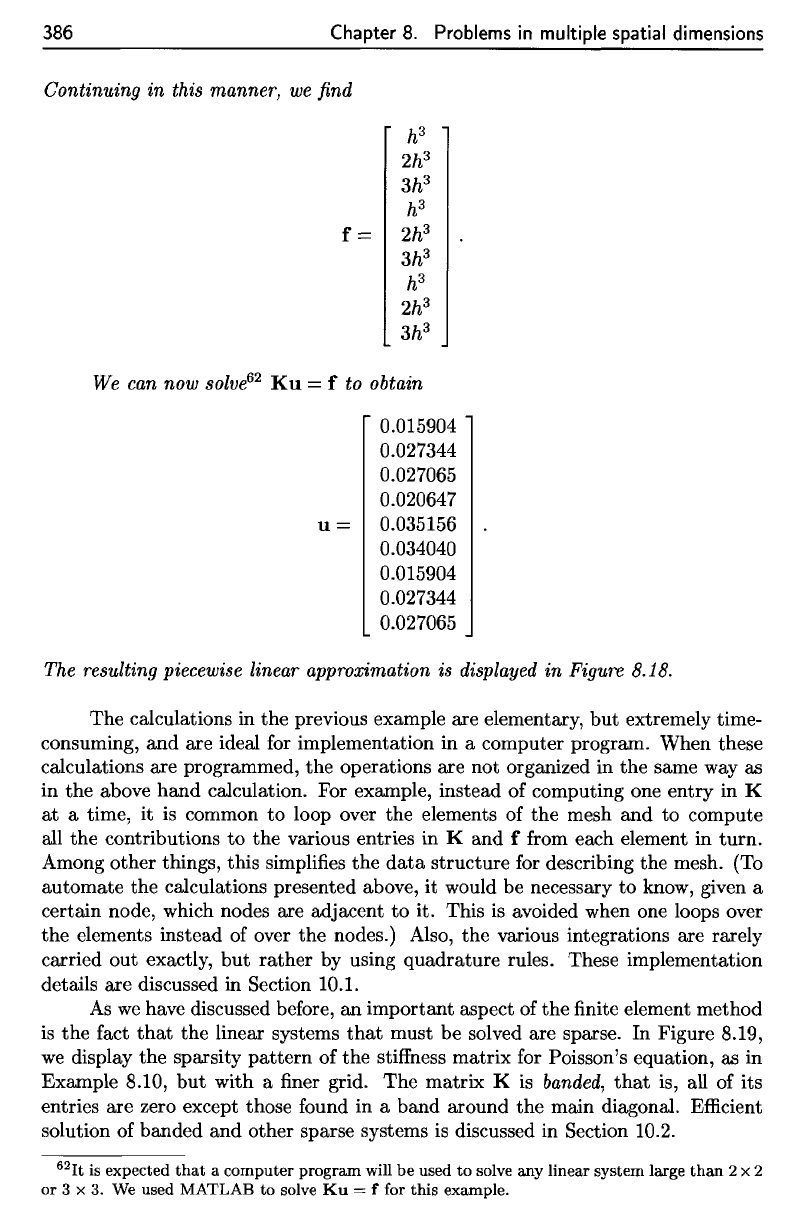
The resulting piecewise linear approximation is displayed in Figure 8.18.
The calculations in
the
previous example are elementary,
but
extremely time-
consuming,
and
are ideal for implementation in a computer program. When these
calculations are programmed,
the
operations are not organized in the same way as
in the above hand calculation. For example, instead of computing one entry in K
at
a time, it
is
common to loop over the elements of the mesh and to compute
all the contributions
to
the various entries in K and f from each element in turn.
Among other things, this simplifies the
data
structure for describing the mesh. (To
automate the calculations presented above, it would be necessary to know, given a
certain node, which nodes are adjacent
to
it. This
is
avoided when one loops over
the
elements instead of over
the
nodes.) Also, the various integrations are rarely
carried out exactly,
but
rather by using quadrature rules. These implementation
details are discussed in Section 10.l.
As
we
have discussed before, an important aspect of
the
finite element method
is
the
fact
that
the linear systems
that
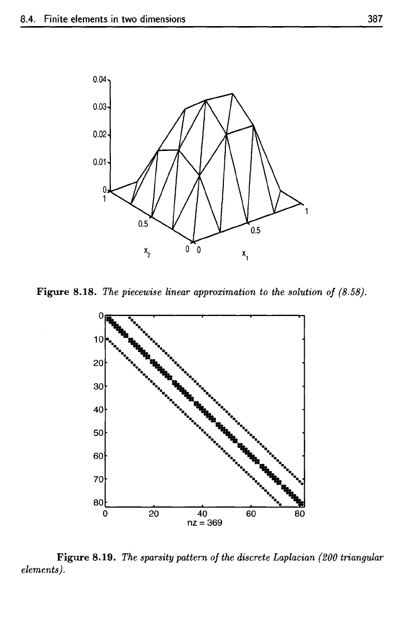
must be solved are sparse. In Figure 8.19,
we
display the sparsity
pattern
of the stiffness matrix for Poisson's equation, as in
Example 8.10,
but
with a finer grid. The matrix K
is
banded,
that
is, all of its
entries are zero except those found in a band around the main diagonal. Efficient
solution of banded and other sparse systems is discussed in Section 10.2.
6
2
It
is expected
that
a
computer
program
will
be
used
to
solve
any
linear system large
than
2 x 2
or
3 X 3. We used MATLAB
to
solve
Ku
= f for
this
example.
8.4.
Finite
elements
in two
dimensions
387
Figure 8.18.
The
piecewise linear approximation
to the
solution
of
(8.58).
Figure
8.19.
The
sparsity
pattern
of
the
discrete Laplacian (200 triangular
elements).
8.4.
Finite elements
in
two dimensions
0.01
o 0
Figure
8.18.
The piecewise linear approximation to the solution
of
{8.58}.
0,
..
10~
,
••••••••
i_.
_.
-.
-.
-.
-.
20
••••
,
••••
e.
_.
-.
-.
30
••••••
,
••••••
-.
-.
.....
,
.....
40
••••
•
•••
•.....•
,
•.....•
50
••••
•
•••
...
,
...
e.
_.
~
~ ~
..•....
,
..•....
-.
-.
70
.~.
:,~~
..
..
..
80
~.
o m
~
~
00
nz
=
369
387
Figure
8.19.
The sparsity pattern
of
the discrete Laplacian {200 triangular
elements}.
