Gockenbach M.S. Partial Differential Equations. Analytical and Numerical Methods
Подождите немного. Документ загружается.

188
Chapter
5.
Boundary value problems
in
statics
(b)
Now
suppose
A
e
R
nxn
is
tridiagonal,
that
is,
suppose
AIJ
— 0
whenever
\i
—
j\ > 1.
About
how
many arithmetic operations does
it
take
to
solve
Ax = b by
Gaussian elimination, assuming
that
the
algorithm takes
advantage
of the
fact
that
most
of the
entries
of A are
already zero?
(The student should work
out a
small example
by
hand
and
count
the
number
of
operation taken
at
each
step.
A
short calculation gives this
operation count
as a
function
of
n.)
(c)
Finally, suppose
that,
on a
certain computer,
it
takes 0.01
s to
solve
a
100 x 100
tridiagonal linear system
by
Gaussian elimination.
How
long
will
it
take
to
solve
a
1000
x
1000 system?
A
10000
x
10000 system?
5.6
Piecewise
polynomials
and the
finite
element
method
To
apply
the
Galerkin method
to
solve
a BVP
accurately
and
efficiently,
we
must
choose
a
subspace
V
n
of
C
2
[0,^]
and a
basis
for
V
n
with
the
following
properties:
1. The
stiffness
matrix
K and the
load vector
f can be
assembled
efficiently.
This means
that
the
basis
for
V
n
should consist
of
functions
that
are
easy
to
manipulate,
in
particular, differentiate
and
integrate.
2.
The
basis
for
V
n
should
be as
close
to
orthogonal
as
possible
so
that
K
will
be
sparse. Although
we do not
expect every pair
of
basis
functions
to be
orthogonal (which
would
lead
to a
diagonal
stiffness
matrix),
we
want
as
many pairs
as
possible
to be
orthogonal
so
that
K
will
be as
close
to
diagonal
as
possible.
3. The
true solution
u
of the BVP
should
be
well
approximated
from
subspace
V^,
with
the
approximation becoming arbitrarily good
as n
—>
oo.
We
will
continue
to use the BVP
as our
model problem.
Finite element methods
use
subspaces
of
piece
wise
polynomials;
for
simplicity,
we
will
concentrate
on
piece
wise
linear functions.
To
define
a
space
of
piecewise
linear functions,
we
begin
by
creating
a
mesh
(or
grid)
on the
interval
[0,^]:
The
points
XQ
,
Xi,...,
x
n
are
called
the
nodes
of the
mesh.
Often
we
choose
a
regular
mesh, with
xi
—
ih,
h =
t/n.
A
function
p
:
[0,^]
—>•
R is
piecewise linear (relative
to the
given mesh)
if, for
each
i =
l,2,...,n,
there exist constants
d{,
b{,
with
188
Chapter
5. Boundary value problems
in
statics
(b)
Now
suppose A E
Rnxn
is
tridiagonal,
that
is, suppose
Aij
= a whenever
Ii
- il >
1.
About how many arithmetic operations does
it
take to solve
Ax
= b by Gaussian elimination, assuming
that
the algorithm takes
advantage of the fact
that
most of the entries of A are already zero?
(The student should work
out
a small example by hand and count
the
number of operation taken
at
each step. A short calculation gives this
operation count as a function of n.)
(c)
Finally, suppose
that,
on a certain computer,
it
takes 0.01 s
to
solve a
100 x 100 tridiagonal linear system by Gaussian elimination.
How
long
will
it
take to solve a 1000 x 1000 system? A 10000 x 10000 system?
5.6 Piecewise polynomials and the finite element
method
To apply the Galerkin method to solve a
BVP
accurately and efficiently,
we
must
choose a subspace
Vn
of C
2
[0,
l]
and a basis for
Vn
with the following properties:
1.
The
stiffness matrix K and the load vector f can be assembled efficiently.
This means
that
the basis for
Vn
should consist of functions
that
are easy to
manipulate, in particular, differentiate and integrate.
2.
The
basis for
Vn
should be as close to orthogonal as possible
so
that
K will
be sparse. Although
we
do not expect every pair of basis functions
to
be
orthogonal (which would lead
to
a diagonal stiffness matrix),
we
want as
many pairs as possible
to
be orthogonal so
that
K will be as close
to
diagonal
as possible.
3.
The
true
solution u of the
BVP
should be well approximated from subspace
V
n
,
with the approximation becoming arbitrarily good as n -+
00.
We
will continue
to
use the BVP
d ( du )
-
dx
k(x)
dx
(x) =
f(x),
0 < x <
/!,
u(O)
= 0, (5.49)
u(/!) = a
as our model problem.
Finite element methods use subspaces of piecewise polynomials; for simplicity,
we
will concentrate on piecewise linear functions. To define a space of piecewise
linear functions,
we
begin by creating a
mesh
(or grid) on
the
interval
[0,
l]:
o = Xo <
Xl
< ... <
Xn
= l.
The
points
Xo,
Xl,
...
,
Xn
are called the nodes of
the
mesh. Often
we
choose a regular
mesh, with
Xi
=
ih,
h =
lin.
A function p :
[0,
l]
-+ R
is
piecewise linear (relative
to the given mesh)
if,
for each i = 1,2,
...
,n,
there exist constants
ai,
b
i
,
with
p(x)
=
aiX
+ b
i
for all X E
(Xi-l,Xi).
5.6.
Piecewise
polynomials
and the
finite element method
189
We
now
argue
that
the
subspace
S
n
satisfies
the
three requirements
for an
approx-
imating subspace
that
are
listed above.
Two of the
properties
are
almost obvious:
1.
Since
the
functions
belonging
to
S
n
are
piecewise polynomials, they
are
easy
to
manipulate—it
is
easy
to
differentiate
or
integrate
a
polynomial.
3.
Smooth functions
can be
well-approximated
by
piecewise linear functions.
In-
deed,
in the
days
before
hand-held calculators,
the
elementary transcendental
functions
like
sin
(x)
or
e
x
were given
in
tables.
Only
a finite
number
of
func-
tion values could
be
listed
in a
table;
the
user
was
expected
to use
piecewise
linear interpolation
to
estimate values
not
listed
in the
table.
The
fact
that
smooth
functions
can be
well-approximated
by
piecewise linear
functions
can
also
be
illustrated
in a
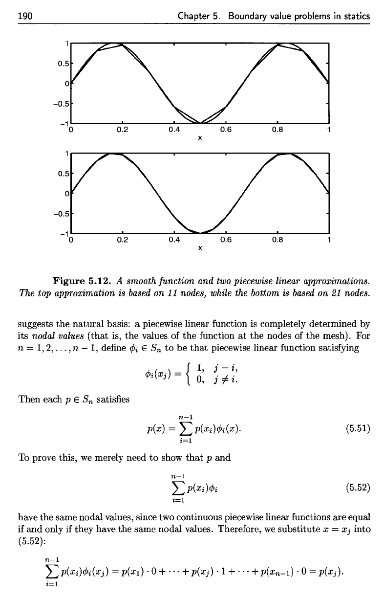
graph. Figure 5.12 shows
a
smooth
func-
tion
on
[0,1]
with
two
piecewise linear approximations,
the first
corresponding
to
n
= 10 and the
second
to
n
= 20.
Clearly
the
approximation
can be
made
arbitrarily good
by
choosing
n
large enough.
In
order
to
discuss
Property
2,
that
the
stiffness
matrix
should
be
sparse,
we
must
first
define
a
basis
for
S
n
.
The
idea
of
piecewise linear interpolation
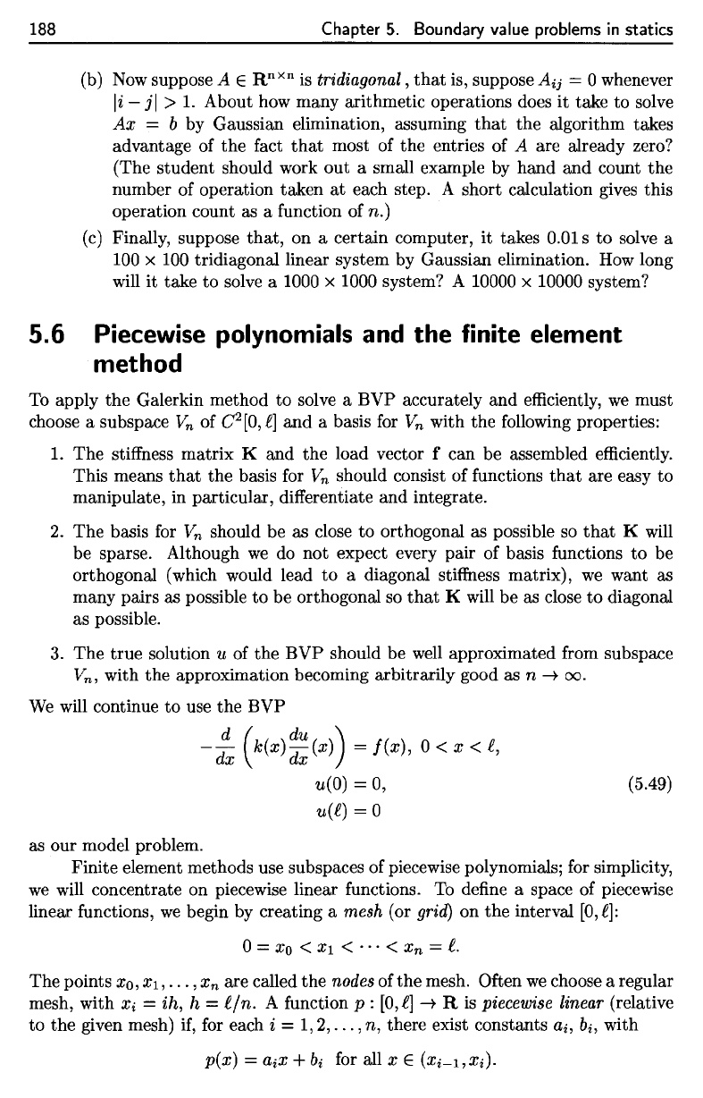
See
Figure 5.11
for an
example
of a
continuous piecewise linear function.
Figure
5.11.
A
piecewise linear function relative
to the
mesh
XQ
=
0.0,31
=
0.25,
x
2
=
0.5,
x
3
=
0.75,
z
4
=
1.0.
We
define,
for a fixed
mesh
on
[0,£],
5.6. Piecewise polynomials
and
the finite element method 189
See Figure 5.11 for
an
example of a continuous piecewise linear function.
0.9
x
Figure
5.11.
A piecewise linear
function
relative to the
mesh
Xo
=
0.0,
Xl
= 0.25,
X2
= 0.5,
X3
= 0.75,
X4
= 1.0.
We
define, for a fixed mesh on
[0,
£],
Sn
=
{p:
[0,£]-+ R : p is continuous
and
piecewise linear,
p(O)
= pee) =
O}.
(5.50)
We now argue
that
the
subspace Sn satisfies
the
three requirements for an approx-
imating subspace
that
are listed above. Two of
the
properties are almost obvious:
1.
Since
the
functions belonging
to
Sn are piecewise polynomials, they are easy
to
manipulate-it
is easy
to
differentiate or integrate a polynomial.
3. Smooth functions can be well-approximated by piecewise linear functions. In-
deed, in
the
days before hand-held calculators, the elementary transcendental
functions like sin (x) or
eX
were given in tables. Only a finite number of func-
tion values could
be
listed in a table;
the
user was expected
to
use piecewise
linear interpolation
to
estimate values not listed in
the
table.
The
fact
that
smooth functions can be well-approximated by piecewise linear
functions can also be illustrated in a graph. Figure 5.12 shows a smooth func-
tion on
[0,
1]
with two piecewise linear approximations,
the
first corresponding
to
n = 10
and
the
second
to
n = 20. Clearly
the
approximation can be made
arbitrarily good by choosing
n large enough.
In
order
to
discuss
Property
2,
that
the stiffness
matrix
should
be
sparse,
we
must first define a basis for Sn.
The
idea of piecewise linear interpolation
190
Chapter
5.
Boundary value problems
in
statics
Figure
5.12.
A
smooth function
and two
piecewise
linear approximations.
The
top
approximation
is
based
on 11
nodes,
while
the
bottom
is
based
on 21
nodes.
suggests
the
natural
basis:
a
piecewise linear function
is
completely determined
by
its
nodal
values
(that
is, the
values
of the
function
at the
nodes
of the
mesh).
For
n
=
1,2,
...,
n
—
1,
define
fa
£
S
n
to be
that
piecewise linear function satisfying
Then each
p
e
S
n
satisfies
To
prove this,
we
merely need
to
show
that
p and
have
the
same nodal values, since
two
continuous piecewise linear functions
are
equal
if
and
only
if
they have
the
same nodal values. Therefore,
we
substitute
x =
Xj
into
(5.52):
190
Chapter
5. Boundary value problems
in
statics
x
0.2
x
Figure
5.12.
A smooth function and two piecewise linear approximations.
The top approximation is based on 11 nodes, while the bottom is based on
21
nodes.
suggests the natural basis: a piecewise linear function
is
completely determined by
its
nodal values (that is, the values of
the
function
at
the nodes of the mesh). For
n = 1,2,
...
, n -
1,
define ¢i E Sn
to
be
that
piecewise linear function satisfying
Then each
p E Sn satisfies
.+.
( )
{I,
j =
i,
<pi
Xj
= 0 .
..J..
, J
r~·
n-l
p(x) =
~p(Xi)¢i(X).
i=l
To
prove this,
we
merely need
to
show
that
p and
n-l
~P(Xi)¢i
i=l
(5.51)
(5.52)
have the same nodal values, since two continuous piecewise linear functions are equal
if
and
only if they have the same nodal values. Therefore,
we
substitute x =
Xj
into
(5.52):
n-l
~P(Xi)¢i(Xj)
=
p(xd·
0 + ... +
p(xj)·l
+ ... +
p(xn-d·
0 = p(Xj).
i=l
5.6.
Piecewise
polynomials
and the
finite
element
method
191
Then,
in
particular,
This
implies
that
all of the
coefficients
c\,
c^,...,
c
n
_i
are
zero,
so
{(f>i,
0
2
,
• • •
?
(f>n-i}
is
a
linearly independent
set.
A
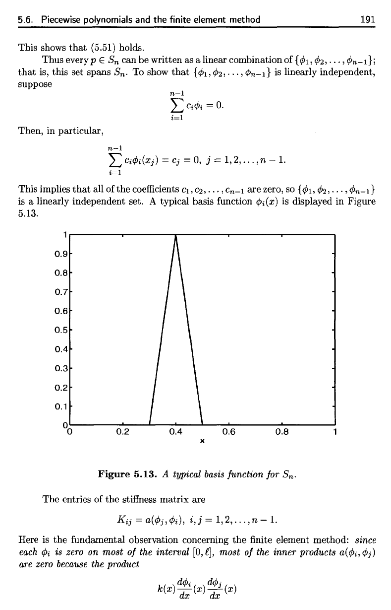
typical basis
function
(f)i(x)
is
displayed
in
Figure
5.13.
Here
is the
fundamental observation concerning
the finite
element method: since
each
fa is
zero
on
most
of the
interval
[0,£],
most
of the
inner products
a(0j,^>j)
are
zero
because
the
product
This shows
that
(5.51) holds.
Thus
every
p 6
S
n
can be
written
as a
linear combination
of
{</»i,
02,
• •
•,
0n-i}
5
that
is,
this
set
spans
S
n
.
To
show
that
{0i,
<fe,
• •
•,
<^n-i}
is
linearly independent,
suppose
Figure 5.13.
A
typical
basis
function
for
S
n
.
The
entries
of the
stiffness
matrix
are
5.6.
Piecewise
polynomials
and
the finite element method
191
This shows
that
(5.51) holds.
Thus every
p E Sn can be written as a linear combination of {
(/J!,
¢2,
...
,
¢n-1};
that
is, this set spans Sn. To show
that
{¢1,
¢2,
...
,
¢n-1}
is
linearly independent,
suppose
n-1
LCi¢i
=
0.
i=1
Then, in particular,
n-1
LCi¢i(Xj)
=
Cj
=
0,
j = 1,2,
..
.
,n-l.
i=1
This implies
that
all of
the
coefficients
C1,
C2,
...
, C
n
-1
are zero, so {
¢1,
¢2,
...
,
¢n-1}
is
a linearly independent set. A typical basis function ¢i(X) is displayed in Figure
5.13.
0.9
0.8
0.7
0.6
0.5
0.4
0.3
0.2
0.2
0.6 0.8
x
Figure
5.13.
A typical basis function for Sn.
The
entries of
the
stiffness
matrix
are
Kij=a(¢j,¢i),
i,j=1,2,
...
,n-l.
Here is
the
fundamental observation concerning
the
finite element method: since
each
¢i is zero on
most
of
the interval
[O,fJ,
most
of
the
inner
products
a(¢i,¢j)
are zero because the product
192
Chapter
5.
Boundary
value
problems
in
statics
is
zero. Therefore,
the
matrix
K
turns
out to be
tridiagonal,
that
is, all of its
entries
are
zero except (possibly) those
on
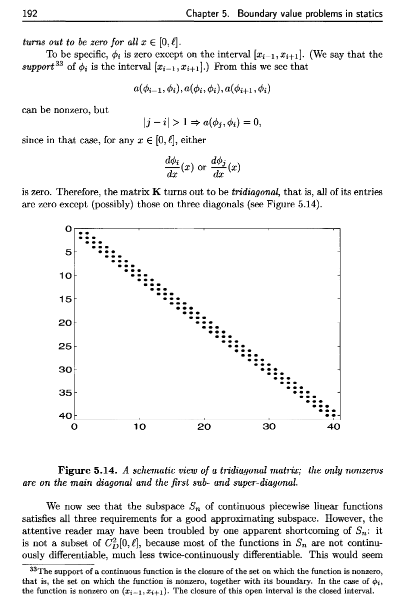
three diagonals (see Figure 5.14).
Figure
5.14.
A
schematic
view
of
a
tridiagonal
matrix;
the
only
nonzeros
are
on the
main
diagonal
and the first
sub-
and
super-diagonal.
We
now see
that
the
subspace
S
n
of
continuous piecewise linear
functions
satisfies
all
three requirements
for a
good approximating subspace. However,
the
attentive reader
may
have been troubled
by one
apparent shortcoming
of
S
n
-
it
is
not a
subset
of
Cf>[0,^],
because most
of the
functions
in
S
n
are not
continu-
ously
differentiate,
much less
twice-continuously
differentiable.
This would seem
33
The
support
of a
continuous
function
is the
closure
of the set on
which
the
function
is
nonzero,
that
is, the set on
which
the
function
is
nonzero, together with
its
boundary.
In the
case
of
</>i,
the
function
is
nonzero
on
(xi-i,Xi+i).
The
closure
of
this open interval
is the
closed interval.
turns
out to be
zero
for all x €
[0,^].
To
be
specific,
fa is
zero except
on the
interval
[ori_i,£i+i].
(We say
that
the
support
33
of fa is the
interval
[xj_i,Xj+i].)
From
this
we see
that
can be
nonzero,
but
since
in
that
case,
for any x
G
[O,/],
either
192
Chapter
5.
Boundary value problems
in
statics
turns out to
be
zero for all x E
[0,
fl·
To
be specific,
¢i
is
zero except on
the
interval
[Xi-l,
Xi+l].
(We
say
that
the
support
33
of
¢i
is
the interval
[Xi-l,
Xi+1].)
From this
we
see
that
can be nonzero,
but
Ii -
il
> 1
=:?
a(¢j,
¢i)
=
0,
since in
that
case, for any x E
[0,
f], either
d¢i
()
d¢j ( )
-x
or-x
dx dx
is
zero. Therefore, the matrix K turns out
to
be tridiagonal,
that
is, all of its entries
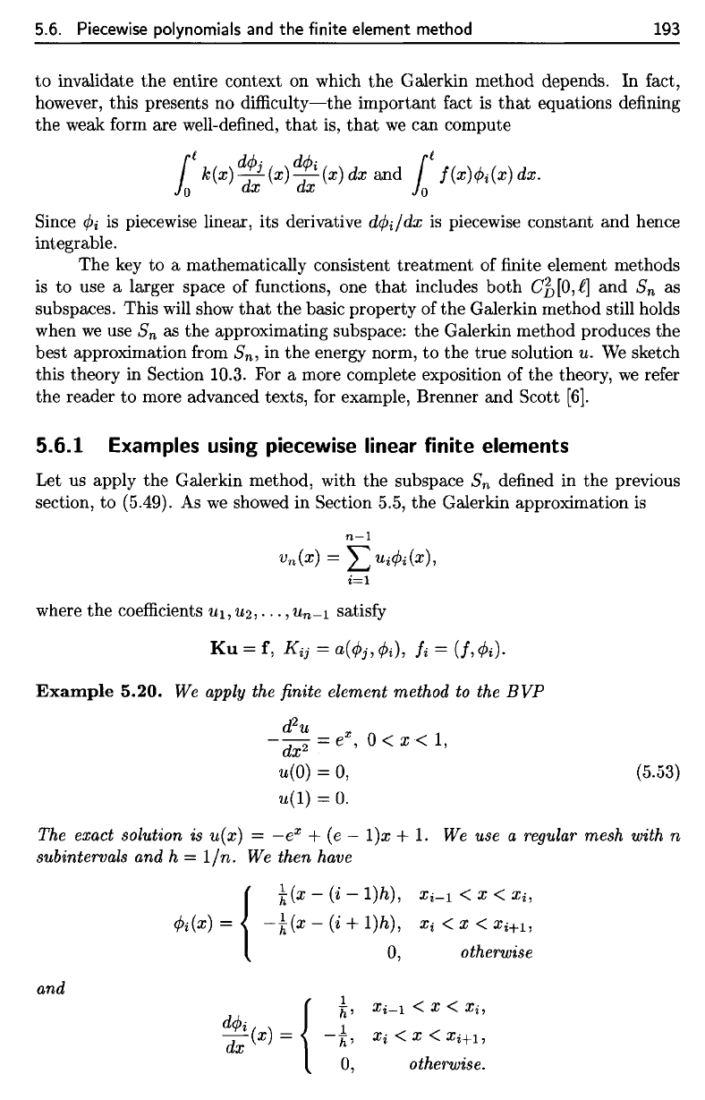
are zero except (possibly) those on three diagonals (see Figure 5.14).
o
••
...
5
10
15
20
25
30
35
...
...
...
...
...
...
...
...
...
...
..
.
...
...
•••
...
...
...
...
•••
...
...
•••
...
•••
...
...
...
...
40L-
________
~
________
~
__________
~
________
~
o
10
20
30
40
Figure
5.14.
A schematic view
of
a tridiagonal matrix; the only nonzeros
are
on the
main
diagonal and the first sub- and super-diagonal.
We
now see
that
the
subspace Sn of continuous piecewise linear functions
satisfies all three requirements for a good approximating subspace. However, the
attentive reader may have been troubled by one apparent shortcoming of Sn: it
is
not a subset of C1[0, f], because most of the functions in Sn are not continu-
ously differentiable, much less twice-continuously differentiable. This would seem
33The
support
of a continuous function is
the
closure of
the
set on which
the
function is nonzero,
that
is,
the
set on which the function is nonzero, together with
its
boundary.
In
the
case
of
ci>;,
the function is nonzero on
(Xi-I,Xi+ll.
The
closure of
this
open interval is the closed interval.
Since
<fo
is
piecewise linear,
its
derivative
dfa/dx
is
piecewise constant
and
hence
integrable.
The key to a
mathematically consistent treatment
of finite
element methods
is
to use a
larger space
of
functions,
one
that
includes both
Cf)[0,l]
and
S
n
as
subspaces. This
will
show
that
the
basic property
of the
Galerkin method still holds
when
we use
S
n
as the
approximating subspace:
the
Galerkin method produces
the
best approximation
from
S
n
,
in the
energy norm,
to the
true solution
u. We
sketch
this theory
in
Section 10.3.
For a
more complete exposition
of the
theory,
we
refer
the
reader
to
more advanced texts,
for
example, Brenner
and
Scott
[6].
5.6.1 Examples using piecewise
linear
finite
elements
Let
us
apply
the
Galerkin method, with
the
subspace
S
n
defined
in the
previous
section,
to
(5.49).
As we
showed
in
Section 5.5,
the
Galerkin approximation
is
5.6. Piecewise polynomials
and the
finite
element
method
193
to
invalidate
the
entire context
on
which
the
Galerkin method depends.
In
fact,
however,
this presents
no
difficulty—the
important
fact
is
that
equations
defining
the
weak
form
are
well-defined,
that
is,
that
we can
compute
where
the
coefficients
MI,
U2,
• •
•,
w
n
-i
satisfy
Example
5.20.
We
apply
the finite
element method
to the BVP
The
exact solution
is
u(x]
=
—e
x
+ (e — l)x + 1. We use a
regular
mesh with
n
subintervals
and
h
=
l/n.
We
then have
5.6.
Piecewise
polynomials
and
the finite element method
193
to
invalidate the entire context on which
the
Galerkin method depends. In fact,
however, this presents no
difficulty-the
important fact
is
that
equations defining
the weak form are well-defined,
that
is,
that
we
can compute
Since
cPi
is
piecewise linear, its derivative dcPddx
is
piecewise constant and hence
integrable.
The key to a mathematically consistent treatment of finite element methods
is
to use a larger space of functions, one
that
includes
both
C'b
[0,
f] and Sn as
subspaces. This will show
that
the basic property of
the
Galerkin method still holds
when
we
use Sn as the approximating subspace: the Galerkin method produces the
best approximation from
Sn, in
the
energy norm,
to
the true solution u.
We
sketch
this theory in Section 10.3. For a more complete exposition of the theory,
we
refer
the reader
to
more advanced texts, for example, Brenner and Scott
[6].
5.6.1 Examples
using
piecewise linear finite elements
Let us apply
the
Galerkin method, with the subspace Sn defined in the previous
section, to (5.49).
As
we
showed in Section 5.5, the Galerkin approximation
is
n-l
vn(x) = L
UicPi(X),
i=l
where
the
coefficients
Ul,
U2,
...
, Un-l satisfy
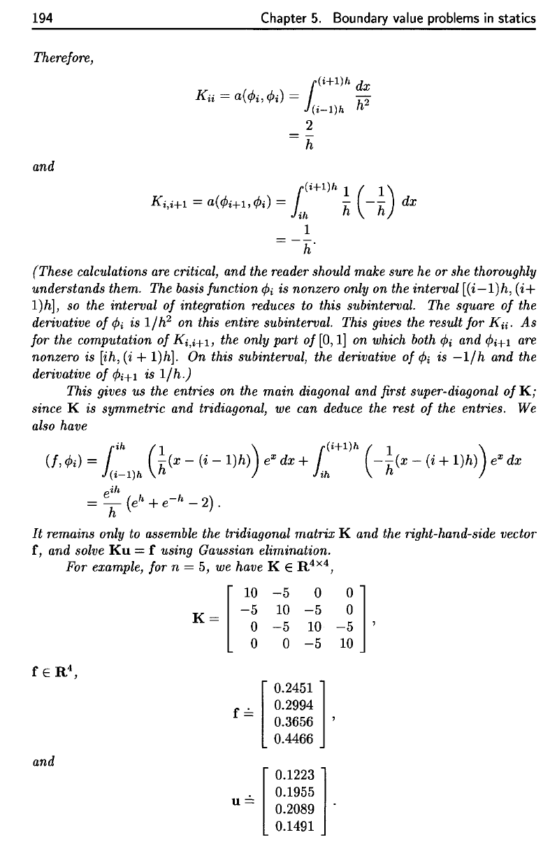
Example
5.20.
We
apply the finite element method to the
BVP
d
2
u
-
dX2
=
eX,
0 < x <
1,
u(O)
= 0,
u(l)
=
O.
(5.53)
The exact solution is
u(x)
=
-ex
+
(e
-
l)x
+
1.
We use a regular mesh with n
subintervals and h =
lin.
We then have
{
~(x
- (i
-l)h),
Xi-l
< x <
Xi,
cPi(X)
=
--k(x
- (i +
l)h),
Xi
< x <
Xi+l,
0,
otherwise
and
1
Xi-l
< X <
Xi,
II'
d¢i(x)
~
{
1
Xi
< X <
Xi+1,
dx
-II'
0,
otherwise.
194
Chapter
5.
Boundary value problems
in
statics
Therefore,
and
(These calculations
are
critical,
and the
reader should make sure
he or she
thoroughly
understands
them.
The
basis
function
fa is
nonzero
only
on the
interval
[(i
—
l)h,
(i+
l)h],
so the
interval
of
integration reduces
to
this subinterval.
The
square
of the
derivative
of fa is
l/h
2
on
this entire subinterval. This gives
the
result
for
KH.
As
for
the
computation
of
Ki^+i,
the
only
part
of
[0,1]
on
which
both
fa and fa+i are
nonzero
is
[ih,(i
+
l)h].
On
this subinterval,
the
derivative
of fa is
—l/h
and the
derivative
of fa
+
i is
l/h.)
This
gives
us the
entries
on the
main
diagonal
and first
super-diagonal
ofK;
since
K is
symmetric
and
tridiagonal,
we can
deduce
the
rest
of the
entries.
We
also
have
It
remains
only
to
assemble
the
tridiagonal matrix
K and the
right-hand-side vector
f,
and
solve
Ku = f
using Gaussian
elimination.
For
example,
for n = 5, we
have
K G
R
4x4
;
194 Chapter
5.
Boundary value problems
in
statics
Therefore,
l
(Hl)h
dx
Kii =
a(¢i'
¢i)
= h
2
(i-l)h
2
=
h
and
r(Hl)h
1 (
1)
K
i
,Hl
=
a(¢Hl,
¢i)
= J
ih
h
-h
dx
1
-h'
(These calculations
are
critical, and the reader should make sure he or she thoroughly
understands them. The basis function
¢i
is nonzero only on the interval
[(
i-I)
h, (i +
l)h],
so
the interval
of
integration reduces to this subinterval. The square
of
the
derivative
of
¢i
is
I1h
2
on this entire subinterval. This gives the result for K
ii
.
As
for the computation
of
K
i
,Hl,
the only part
of
[0,
1]
on which both
¢i
and
¢Hl
are
nonzero is
[ih,
(i + l)h]. On this subinterval, the derivative
of
¢i
is
-l/h
and the
derivative
of
¢Hl
is
Ilh.)
This gives us the entries on the main diagonal and first super-diagonal
of
K;
since K is symmetric and tridiagonal, we can deduce the rest
of
the entries. We
also have
(I,
¢i)
=
l~h
(~(X
-(i -
l)h))
eX
dx
+
(i+l)h
(-~(X
-(i +
l)h))
eX
dx
(,-I)h
J
ih
e
ih
= -
(e
h
+ e-
h
-
2)
.
h
It
remains only to assemble the tridiagonal matrix K and the right-hand-side vector
f,
and solve
Ku
= f using Gaussian elimination.
and
For example, for n
= 5,
we
have K E R
4X4
,
[
10
-5
0 0 ]
=
-5
10
-5
0
K 0
-5
10
-5
'
o 0
-5
10
f
==
0.2994
[
0.2451 ]
0.3656 '
0.4466
[
0.1223]
==
0.1955
u
0.2089'
0.1491
5.6. Piecewise polynomials
and the
finite
element method
195
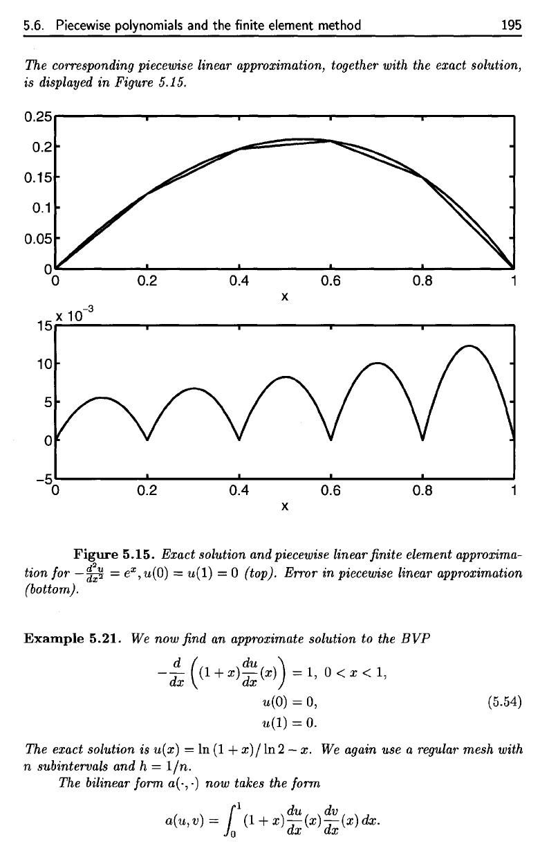
The
corresponding piecewise linear approximation, together with
the
exact
solution,
is
displayed
in
Figure
5.15.
Figure
5.15. Exact solution
and
piecewise linear
finite
element approxima-
tion
for
-£-%
=
e
x
,u(Q)
=
w(l)
= 0
(top). Error
in
piecewise linear approximation
(bottom).
Example
5.21.
We now find an
approximate solution
to the
BVP
The
exact solution
is
u(x)
=
In
(1 +
x)/ln2
—
x. We
again
use a
regular mesh with
n
subintervals
and h —
l/n.
The
bilinear form
a(-,
•) now
takes
the
form
5.6.
Piecewise
polynomials
and
the finite element method
195
The corresponding piecewise linear approximation, together with the exact solution,
is displayed
in
Figure 5.15.
0.25r-----.....,...-----r-------,----.....,------,
-3
15 X 10
x
0.6 0.8 1
-5~------~--------~--------~--------~------~
o 0.2 0.4 0.6 0.8 1
X
Figure
5.15.
Exact solution and piecewise linear finite element approxima-
tion for
-~
=
eX,
u(O)
=
u(l)
= 0 (top). Error
in
piecewise linear approximation
(bottom).
Example
5.21.
We now find an approximate solution to the
BVP
d ( dU)
--
(l+x)-(x)
=1,
dx
dx
u(O)
= 0,
u(l)
=
O.
0<
x < 1,
(5.54)
The exact solution is
u(x)
= In
(1
+
x)/In2
- x. We again use a regular mesh with
n subintervals and h =
lIn.
The bilinear form
a(·,·)
now takes the form
(l
du dv
a(u,v)
=
10
(1
+
x)dx(x)dx(x)dx.
196
Chapter
5.
Boundary value problems
in
statics
We
obtain
and
It
remains
only
to
assemble
the
tridiagonal
matrix
K and the
right-hand-side vector
f,
and
solve
Ku = f
using Gaussian elimination.
For
example,
if
n —
5,
the
matrix
K is 4 x 4,
and
f is a
4-vector,
The
resulting
u is
The
piecewise
linear approximation, together with
the
exact solution,
is
shown
in
Figure
5.16.
Fundamental
issues
for the
finite
element method are:
As in the
previous example, these calculations
suffice
to
determine
K. We
also
have
How
fast does
the
approximate
solution converge
to the
true
solution
as n
-»
oo?
196
Chapter
5.
Boundary value problems
in
statics
We obtain
l
(i+I)h
( 1 )
a(¢i,
¢i)
=
(1
+ x) h
2
dx
(i-1)h
2(ih
+
1)
h
and
1
(i+1)h
( 1 (
1))
a(¢i+1'
¢i)
=
ih
(1
+
x)h
-h
dx
h +
2ih
+ 2
2h
As
in the previous example, these calculations suffice to determine K. We
also
have
l
ih
(1
)
1(i+
1
)h (
1 )
(1,
¢i)
=.
h(x
- (i -
l)h)
dx + .
-h(x
- (i +
l)h)
dx
(.-1)h
.h
=h.
It
remains only to assemble the tridiagonal matrix K and the right-hand-side vector
f, and solve
Ku
= f using Gaussian elimination.
For example,
if
n =
5,
the matrix K
is
4 x 4,
and f
is
a 4-vector,
The resulting
u is
[
12
13
K-
-2
- 0
o
f=
13
0
-2
14
15
-2
15
16
-2
0
17
-2
[
1/5
)
1/5
1/5
.
1/5
==
0.0851
[
0.0628]
u
0.0778'
0.0479
)),
18
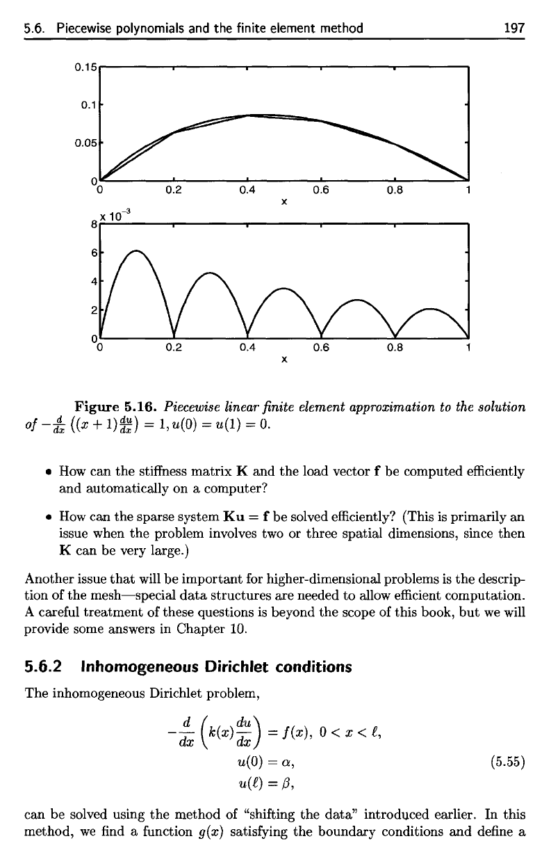
The piecewise linear approximation, together with the exact solution, is shown in
Figure 5.16.
Fundamental issues for
the
finite element method are:
• How fast does
the
approximate solution converge
to
the
true
solution as n
-+
oo?
5.6.
Piecewise
polynomials
and the
finite
element method
197
Figure
5.16.
Piecewise
linear
finite
element
approximation
to the
solution
• How can the
stiffness
matrix
K and the
load vector
f be
computed
efficiently
and
automatically
on a
computer?
• How can the
sparse system
Ku = f be
solved
efficiently?
(This
is
primarily
an
issue when
the
problem involves
two or
three
spatial
dimensions, since then
K can be
very large.)
Another issue
that
will
be
important
for
higher-dimensional
problems
is the
descrip-
tion
of the
mesh—special
data
structures
are
needed
to
allow
efficient
computation.
A
careful
treatment
of
these questions
is
beyond
the
scope
of
this book,
but we
will
provide some answers
in
Chapter
10.
5.6.2
Inhomogeneous
Dirichlet
conditions
The
inhomogeneous Dirichlet problem,
can be
solved using
the
method
of
"shifting
the
data"
introduced
earlier.
In
this
method,
we find a
function
g(x]
satisfying
the
boundary conditions
and
define
a
5.6.
Piecewise
polynomials
and
the finite element method
197
0.15..--------r----,.------,----...,-------.
0.1
0.4
x
0.6
O.B
x
Figure
5.16.
Piecewise linear finite element approximation
to
the solution
of
-/x
((x +
l)~~)
= 1,u(O) =
u(l)
= O .
• How can the stiffness matrix K and the load vector f be computed efficiently
and automatically on a computer?
•
How
can the sparse system
Ku
= f be solved efficiently? (This
is
primarily an
issue when
the
problem involves two or three spatial dimensions, since then
K can be very large.)
Another issue
that
will be important for higher-dimensional problems
is
the
descrip-
tion of the
mesh-special
data
structures are needed
to
allow efficient computation.
A careful treatment of these questions
is
beyond the scope of this book,
but
we
will
provide some answers in Chapter
10.
5.6.2 Inhomogeneous Dirichlet conditions
The inhomogeneous Dirichlet problem,
d (
dU)
-
dx
k(x)
dx
=
f(x),
0 < x <
£,
u(O)
=
0:,
(5.55)
u(£)
=
/3,
can be solved using
the
method of "shifting the data" introduced earlier. In this
method,
we
find a function g(x) satisfying the boundary conditions and define a
