Genshiro Kitagawa. Introduction to Time Series Modeling (Введение в моделирование временных рядов)

Подождите немного. Документ загружается.

MONTE CARLO FILTE R 229

standard normal distribution N(0,1), respectively. The initial state dis-

tribution p

) is assumed to follow the standard normal d istribution.

However, it is evident that normality of the distribution is not essential

for the Monte Carlo ﬁltering m ethod.

Under the above-mentioned assumptions, the one-step-ahead predic-

tive distribution p(x

) and the ﬁlter p(x

) were obtained. Here, a

small num ber of par ticles was used, that is, m was set to m = 100, in or-

der to make features of the illustrations clearly visible. In actual co mpu-

tations, however, we use a large number of particles for approximation.

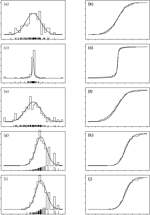
The curve in Figure 15 .3(a) shows the assumed distribution of the

initial state p

). The vertical lines show the locations of 100 real-

izations generated from p

), and the histogram, which was o btained

from these particles, approximates the probability density function. The

bold curve in plot (b) d epicts the true distribution function of the initial

state and the fainter curve shows the empirical distribution function ob-

tained from the particles shown in plot (a). Similar to these plots, plots

the cumulative distribution, together with its empirica l counterpart of

the system noise.

Plots (e) and (f) illustrate the predictive distribution, p(x

). The

curve in plot ( e) shows the “true” probability function obtained by nu-

merical integration of the two density functions of plots (a) and (c). Plot

(f) shows the “true” cumulative distribution function obtained b y inte-

grating the de nsity function in plot (e). On the other hand, the vertical

lines in plot (e) indicate the location of the particles p

( j)

obtained by sub-

stituting a pair of particles shown in plots (a) and (c) into the eq uation

(D.4). The h istogram deﬁned by the particles p

(1)

,.. ., p

(m)

approximates

the true density function shown in plot (e). The empirical distribution

function and the true distribution function are shown in plot (f).

The cu rve in plot (g) shows the ﬁlter d ensity function obtained from

the non-Gaussian ﬁlter using the equation (14.5), when the observation

= 2 is given. With respect to plot (g), the particles are lo cated in the

same place as plot (e); however, the heights of the lines are pr oportional

to the likelihood of the particle

( j)

. Different from plot (f), the c umula-

tive distribution function in plot (h) approximates the ﬁlter distribution,

although the steps of plot (h ) are located identically to those of plot (f).

Plot ( i) shows the locatio ns of the particles, the histogram a nd th e exact

ﬁlter distribution after re-sampling. Further it can be seen that the den-

sity function and the cumulative distribution function in plots (i) and (j)

are reasonable approximations to plots (g) and (h), respectively.

230 THE SEQUENTIAL MONTE CARLO FILTER

Figure 15.3 One step of the Monte Carlo ﬁlter. The ﬁgures in the left-hand col-

umn illustrate the probability density functions, 100 realizations and the his-

togram, respectively, and the ﬁgures in the right-hand column depict the dis-

tribution functions and the empirical distribution functions obtained from the

realizations, respectively. (a) and (b): the initial state distributions. (c) and (d):

the system noise distribution. (e) and (f): the one-step-ahead predictive distribu-

tions. (g) and (h): the ﬁlter distributions. (i) and (j): the ﬁlter distributions after

re-sampling.

MONTE CARLO SMOOTHING METHOD 231

15.3 Monte Carlo Smoothing Method

The Monte Carlo ﬁlter method presented in the previous section, can

be further extended to create a smoothing algorithm by preserving pa st

particles. In the following, the vector of the particles (s

( j)

1|n

,.. ., s

( j)

n|n

)

de-

notes the j-th realization from the n-dimensional join t distribution func-

tion p(x

,.. ., x

To achieve the objective of smoothing, it is necessary only to modify

Step 2(d) of the algorithm discussed in Section 15.2 as follows.

(d-S) For i = 1,... ,m, by re-sampling the n-dimensional vector

( j)

1|n−1

,.. .,s

( j)

n−1|n−1

, p

( j)

)

, generate (s

( j)

1|n

,.. ., s

( j)

n−1|n

( j)

n|n

)

In this modiﬁcation, by re-sampling {(s

1|n−1

,.. ., s

( j)

n−1|n−1

, p

( j)

)

j = 1,. .. ,m} with the same weights as used in step (2)(ii) of subsec-

tion 15.2.3, ﬁxed-interval smoothing for a nonlinear n on-Gaussian state-

space model can be achieved (Kitagawa (1996)).

In actual computation, however, since a ﬁnite number of particles

(m particles) is repeatedly re-sampled, the number of different parti-

cles gradually decreases and then the weights become concentr ated on

a small numb e r of particles, thus causing the shape of the distribution

to ﬁnally collapse. Consequently, in terms of the smoothing algorithm, a

modiﬁcation for Step (d-S) should be carried out as follows:

(d-L) For j = 1,... ,m, generate (s

( j)

n−L|n

,.. ., s

( j)

n−1|n

( j)

n|n

). Here, L is

assumed to be a ﬁxed integer, usually less than 30, and f

( j)

n|n

by re-sampling (s

( j)

n−L|n−1

, ..., s

( j)

n−1|n−1

, p

( j)

Then, it is interesting that this modiﬁed algorithm turns out to corre-

spond to the L-lag ﬁxed-lag smoothing algorithm. If L is ﬁxed too large,

the ﬁxed- lag smoother p(x

n+L

) precisely approximates the ﬁxed-

interval smoother p(x

). On the other hand, the distribution deter-

mined by x

(1)

n|n+L

,.. ., x

(m)

n|n+L

is rather remote from p(x

n+L

). Therefore,

L should be taken not so large, i.e., L = 20 or 30.

The following example shows the resu lts of state estimation by the

Monte Carlo ﬁlter for the artiﬁcially generated time series shown in Fig-

ure 14.1. The estimation is carried out by applyin g a ﬁrst order trend

model;

= x

n−1

+ v

= x

+ w

, (15.11)

232 THE SEQUENTIAL MONTE CARLO FILTER

- 3

- 2

- 1

1 10 1 2 0 1 3 0 1

- 3

- 2

- 1

0 1 00 2 0 0 300

-3

-2

-1

0 100 200 300

-3

-2

-1

0 100 200 300

(a)

(b)

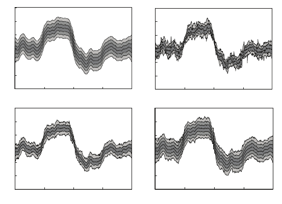
Figure 15.4 The results of the Monte Carlo ﬁlter: (a) the exact ﬁlter distribution

using a K alman ﬁlter. (b) – (d) the ﬁxed-lag (L = 20) smoothed densities ((b)

m = 100, (c) m = 1000, (d) m = 10, 000) with a Monte Carlo ﬁlter.

where w

is a Gaussian white noise with mean 0 and variance

. For

the system noise, two models are considered, namely, a Gaussian distri-

bution and a Cauchy distribution.

Figure 15.4 (a) depicts the exact ﬁlter d istribution ob ta ined by the

Kalman ﬁlter when th e system noise is Gaussian. The bold c urve in the

middle shows the mean of the d istribution and the three gray areas illus-

trate ±1

, ±2

and ±3

conﬁdence intervals.

On the other hand, plots (b), (c) and (d) show the ﬁxed-lag (L =

20) smoothed densities obtained by using m = 100,1000 and 10,000

particles, respectively. The dark gr ay area shows the ±1

interval and

the light gray area shows the ±2

intervals. In plot (d), the ±3

interval

is also shown.

For m = 100 in plot (b), although general tendencies of the distribu-

tional change of plot (a) are captured, large variation is seen which indi-

cates that the estimate is not particularly good. However, as th e number

of particles increases, more accurate ap proximations to the “true” dis-

tribution are obtained. In particular, for m = 10,0 00 shown in plot (d),

NONLINEAR SMOOTHING 233

-3

-2

-1

0 100 200 300

- 3

- 2

- 1

0 1 0 0 2 0 0 30 0

(a) (b)

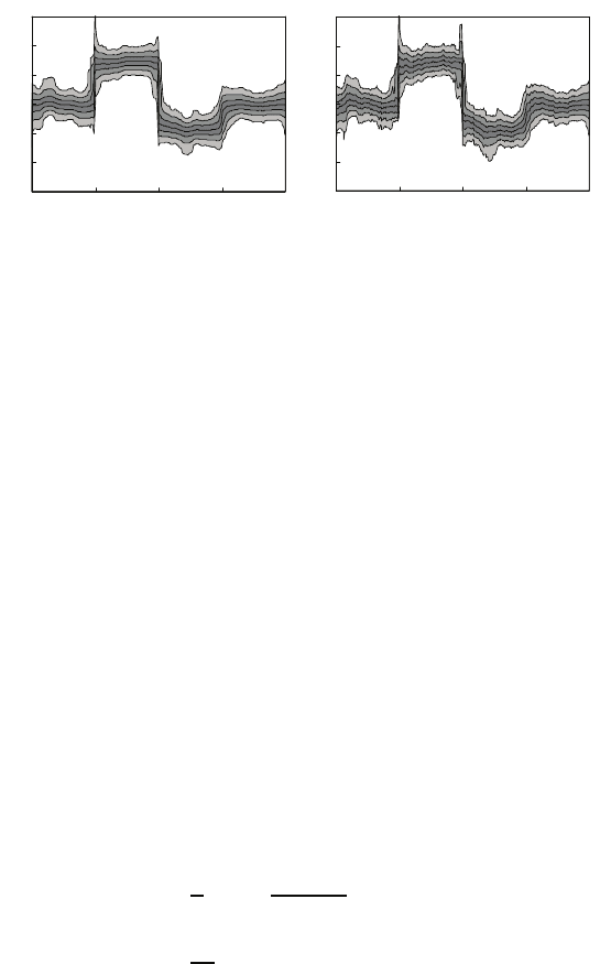
Figure 15.5 Smoothing with Cauchy distribution model: (a) The exact distribu-

tion obtained from the non-Gaussian smoothing algorithm. (b) The results of

Monte Carlo smoothing (m = 10,000).

a very good approximation of the curves are obtained except the ±3

interval of which curves are slightly variable.

Figure 15.5 shows the results when the system noise is assumed to

be a Cauchy distribution. The ﬁgure on the left-hand side depicts the

“exact” results obtained using the non-Gaussian smooth ing algorithm,

which was trea ted in Chapter 1 4. On the other hand, the ﬁgure on the

right-ha nd side depicts the results obtained by Monte Carlo smo othing

with m = 10,000 and L = 20. Although the curves ar e more variable

in comparison with the ﬁgure on the left-hand side, the abrupt changes

around n = 100,200 and 30 0 are captured in a reasonable way. Moreover,

the ±3

interval is also well approximated.

15.4 Nonlinear Smoothing

The Monte Carlo ﬁltering and smoothing algorithms can also be used f or

ﬁltering and smoothin g for the nonlinear state-space model (Kitagawa

(1991)). Figures 15.6 (a) and (b) depict examples of series x

and y

generated by the nonlinear state-sp ace model

n−1

25x

n−1

+ 1

+ 8 cos(1.2n) + v

+ w

, (15.12)

where v

∼ N(0, 1), w

∼ N(0, 10), v

∼ N(0, 5). He re, we consider the

problem of estimating the unknown state x

based on 100 obser vations,

, n = 1, ... ,100. Because o f the nonlinearity and the sinusoidal input

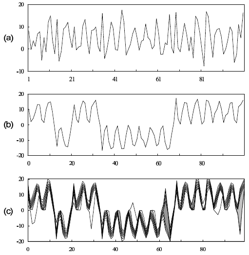
234 THE SEQUENTIAL MONTE CARLO FILTER

Figure 15.6 Nonlinear smoothing: (a) Data y

. (b) Unknown State x

. (c)

Smoothed distribution of x

obtained by the Monte Carlo smoother.

in the system model in equation (15.12), the state x

occasionally shifts

between the positive and negative regions. However, since in the obser-

vation model, the state x

is squared, and x

contamina te d with an obser-

vation noise w

is observed, it is quite difﬁcult to discriminate between

positivity and n egativity of the true state.

It is well known tha t the extended Kalman ﬁlter occasionally diverges

for this model. Figure 15 .6 (c) shows the smoothed posterior distribu-

tion p(x

) obtained by the Monte Calro ﬁlter and smoother. It can be

seen that a quite reasonable estimate of the state x

is obtained with this

method.

The key to the success of the nonlinea r ﬁltering and smoothing is

that the Monte Carlo ﬁlter can reasonably express the non-Gaussian state

densities. Figure 15.7 (a) and (b), respectively, show the marginal pos-

terior state distributions p(x

t+ j

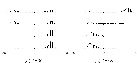
), j = −1,0,1,2, for t = 30 and 48.

NONLINEAR SMOOTHING 235

Figure 15.7 Fixed-point smoothing for t = 30 (left) and t = 48 (right). From top

to bottom, predictive distributions, ﬁlter distri butions, 1-lag smoothers and 2-lag

smoothers.

For both t = 3 0 and 48, the predictive distribution p(x

t−1

) and the ﬁl-

ter distribution p(x

) are b imodal. However, in the 2-lag smoother f or

t = 30, p(x

), the le ft-half of the d istribution disappeared and the

distribution becomes unimodal. The same phenomenon can be seen for

t = 48. In this case, th e r ight peak is higher than the left one in the predic-

tive distribution. However, in the smooth er distributions, the peak in the

right half do main disappears. I n such a situation, the extended Kalman

ﬁlter is very likely to yield an estimate with reverse sign.

Problems

1. Co nsider a model for the Nikkei 225 data shown in Figure 1. 1(g) that

takes into account change s in the trend and the volatility simultan e -

ously.

2. In Monte Carlo ﬁltering, how many particles should we use to in-

crease the accuracy of the estimate 1 0-fold.

3. For the Monte Carlo ﬁlter, if we do not restrict every particle to have

the same weight but allow some to have different weig hts, is it possi-

ble to develop a procedure without re-sampling?

4. Co mpare the amount of information required to be stored to ca rry out

ﬁxed-interval smoothing and ﬁxed-lag smoothing.

Chapter 16

Simulatio n

In this chapter, we ﬁrst explain methods for generating random number s

that follow various distributions. A uniﬁed method for simulating time

series is obtained by using the state-spac e model. Namely, a realization

of white noise can be obta in by generating random numbers that follow

a spec iﬁed distribution. In modeling, a time series model is generally

considered an output of a system with a white noise input. Therefore,

if a time series model is given, we c a n o btain realizations of the sys-

tem by gener a ting a time series that follows the model by using random

numbers.

16.1 Generatio n of Uniform Random Numbers

A sequence of independently generated numbers th at follows a certain

distribution is called a sequence of random numbers or simply random

numbers. In other words, the random numbers are realizations of white

noises. A time series m odel repre sents a time series as a sequence of

realizations of a system with white noise input. Therefore, we can gen-

erate a time series by properly specifying the time ser ies model and the

random numbers, a nd this method is called a simulatio n of a time series

model. In actual computation for simulating a time series, we usually

use pseudo-random numbers generated using an appro priate algorithm.

Normal random numbers, i.e., ra ndom numbers that follow a normal dis-

tribution, are freque ntly ne cessary for simulatin g time series. Such a se-

quence of random numbers is obtained by gener a ting uniform random

numbers, and then transforming them to the speciﬁed distribution.

A well-known conventional method for generating uniform random

numbers is the linear congruence method. With this method, a sequence

of integers I

,··· is generated from

≡ aI

k−1

+ c (mo d m), (16.1)

starting from an initial integer I

237

238 SIMULATION

In particular, for c = 0, this method is called the multiplica tive con-

gruence method. The generated integer I

takes a value in [0,m). There-

fore, I

/m is distributed on [0,1).

However, we note here that since the period of the series generated

by this method is at most m, it is not possible to generate a sequence

of random numbers longer than m. The constants a, c and m have to be

selected carefully, and examples of the combination of constants are

a =1229 c =351750 m =1664501

a =1103515245 c =12345 m = 2

(Knuth (199 7)). The latter combination were used in C language until

1990-th. It is known that if m = 2

, a = 5 (mod m) an d c is an odd num-

ber, then the period of the sequence generated by this algorithm attains

the possible maximum period of m, i.e., it contains all of the numbers

between 0 and m −1 once each.

By the lagged Fibonacci method, the sequence of integers I

is gen-

erated by

n+p

= I

n+q

+ I

(mod m), (16.2)

where m is usually set to 2

(k ia the bit length). Then the generated

series has the period at largest 2

k−1

−1). In the current C langua ge,

p = 31, q = 3, m = 2

are used to attain the period of about 2

In the generalize feedback shift register (GFSR) algorithm (Lewis

and Payne ( 1973)), k -dimensional vector of bina ry sequence is generated

n+p

= I

n+q

⊕I

, (16.3)

where p > q and ⊕ denotes the excu sive OR operation. The integers p

and q are de te rmined so that the polynomial X

+ X

+ 1 is irreducible.

Then, the period of the sequence becomes at largest 2

−1. Some exam-

ples of p and q are p = 521, q = 158 (period 2

521

−1), p = 521, q = 32

(period 2

521

−1) and p = 607, q = 273 (period 2

607

−1).

Twisted GFSR algorithm (Matsu moto and Kurita (1994)) g e nerates

a k-dimensional binary sequence by

n+p

= I

n+q

⊕I

A, (16.4)

where A is a k ×k regular matr ix such as the companion matrix. In

the frequently used TT800 algorithm, p = 25 and q = 7 are used. This

sequnce has the period of 2

−1. Further, Matsumoto an d Nishimura

(1998) developed the Mersenne twister algorithm

n+p

= I

n+q

⊕I

n+1

B ⊕I

A. (16.5 )