Gebali F. Analysis Of Computer And Communication Networks

Подождите немного. Документ загружается.

11.4 Discrete-Time Modeling: Interarrival Time for Bernoulli Traffic 399

The probability that k packets arrive in n time steps is given by the binomial

distribution

p(k) =





n−k

(11.43)

We can think of the interarrival time n between two successive packets as a ran-

dom variable N. This r.v. is discrete for Bernoulli traffic.

The probability p(0) that no packets arrive for at least n consecutive time steps

is given by

p(0) = y

The above equation simply states that we did not get any packets in n time steps.

What happens during time step n + 1 is not specified in the above equation. We

might get a packet or we might not. Notice that for large n, the probability that no

packets arrive diminishes which makes sense.

The above probability is equivalent to the event A : N > n, and we can write

p(A : N > n) = p(0)

= (1 − x)

(11.44)

This equation will help us in the next section to prove the memoryless property

of Bernoulli traffic. However, we proceed here to find the pmf associated with the

interarrival time.

In order to find the pmf associated with the interarrival time, we need to find the

probability that the interarrival time exactly equals n time steps. In other words, our

event now specifies that no packets arrived for n time steps followed by a packet

arrival event at the next step when the time index is n + 1. The desired probability

is given by

p = x (1 − x)

(11.45)

This probability is equal to the pmf of the interarrival time and we can write the

pmf as

p(N = n) = x (1 − x)

(11.46)

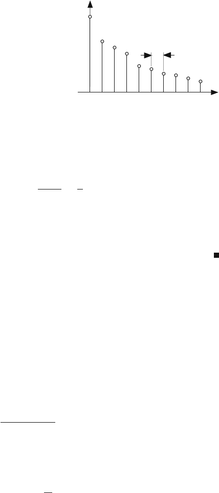
Figure 11.6 illustrates the pmf for the interarrival time of Bernoulli traffic that

has geometric distribution. A simple geometric distribution with one parameter x,

the probability that exactly one packet arrives at the end of time interval n,isshown

in Fig. 11.6.

Example 11.8 Find the average value for the interarrival time of Bernoulli traffic

which is described by the pmf distribution of (11.46).

400 11 Modeling Network Traffic

Fig. 11.6 A simple geometric

distribution with one

parameter x, the probability

that exactly one packet

arrives at the end of time

interval n

p(N = n)

...

012

The average number of time steps between packets n

is given by

∞



n=0

nxy

1 − y

We see that as the probability for the packet arrival decreases (x  1), the aver-

age number of steps between the packets increases as expected. On the other hand,

when x approaches unity, the interarrival time becomes n

≈ 0 as expected. This

indicates that arriving packets have no empty time slots in between them.

Example 11.9 Consider communication channel where packets arrive with an aver-

age data rate of λ

= 2.3×10

packets/s and a burst rate limited only by the line rate,

σ = λ

= 155.52 Mbps. Derive the equivalent binomial distribution parameters and

find the probability that 10 packets arrive in one sample time period of T = 1ms.

The average number of packets received in one time step period is given by

= 2.3 ×10

×10

−3

= 23

which represents the average traffic produced by the source.

The maximum number of packets that could be received in this time is found by

estimating the duration of one packet as determined by the line rate.

⌬ =

8 ×53

155.52 ×10

= 2.7263 ␮s

The maximum number of packets that could be received in 1 ms period is given

= 367

The packet arrival probability per time step is given the equation

= N

11.4 Discrete-Time Modeling: Interarrival Time for Bernoulli Traffic 401

which gives

x =

367

= 0.0627

and of course y = 1 − x = 0.9373.

The probability of 10 cells arriving out of potential N

cells is

p(10) =





−10

= 9.3192 ×10

−4

We note that p(10) as obtained here is almost equal to p(10) as obtained using the

Poisson distribution in Example 11.4.

11.4.1 Realistic Models for Bernoulli Traffic

The Bernoulli distribution and the interarrival time considered in Section 11.4 do not

offer much freedom in describing realistic traffic sources since they contain only one

parameter: x represented the probability that a packet arrived at a given time step.

The minimum value for the interarrival time is zero (i.e., n = 0). This implies that

the time interval between two packet headers could be exactly one time step.

Equation (11.46) can be modified as follows

p(N = n) = x (1 − x)

(n−n

)

(11.47)

Now the traffic distribution can be described by two parameters x and n

.The

parameter n

represents the minimum number of time steps between adjacent pack-

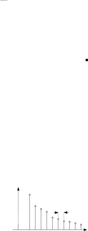
ets. Figure 11.7 illustrates the pmf for the interarrival time of Bernoulli traffic that

has geometric distribution. A simple shifted, or biased, geometric distribution with

two parameters x and n

is shown in Fig. 11.7.

Fig. 11.7 A realistic model

for the geometric distribution

of Bernoulli traffic

interarrival time. The

distribution is described in

terms of two parameters x

and n

p(N = n)

...

402 11 Modeling Network Traffic

11.4.2 Memoryless Property of Bernoulli Traffic

Assume that n is the number of time steps between arriving packets. It is obvious

that the value of n shows random variations from one packet to another. Define N

as the random variable associated with n. The memoryless property of the interar-

rival time for Bernoulli traffic is defined using the following conditional probability

expression for discrete random variables

p(N > n + m|N > n) = p(N > m) for all n, m > 0 (11.48)

Basically, this equation states that the probability that a packet arrives after a time

n + m, given that no packets arrived up to time n, does not depend on the value of

n. It depends only on m.

From (11.44), we could write

p(n) = (1 − x)

(11.49)

where x is the packet arrival probability during one time step. Changing the time

value from n to n + m, we get

p(n + m) = (1 −x)

n+m

(11.50)

Equation (11.48) is a conditional probability, and we can write it as

p(A|B) =



(



p(B)

(11.51)

where the events A and B are defined as

A : N > n +m (11.52)

B : N > n (11.53)

But A

(

B = A since m > 0, which implies that if event A took place, then

event B has also taken place. Thus we have

p(N > n + m|N > n) =

p(A)

p(B)

(11.54)

(1 − x)

n+m

(1 − x)

(11.55)

= (1 − x)

(11.56)

= p(N > m) (11.57)

Thus we have proved that the interarrival time for Bernoulli traffic is memoryless.

11.4 Discrete-Time Modeling: Interarrival Time for Bernoulli Traffic 403

11.4.3 Realistic Model for Bernoulli Traffic

The interarrival time considered in Section 11.4 does not offer much freedom in

describing realistic traffic sources since it contains only one parameter: x the prob-

ability that a packet arrives at a certain time step. As mentioned, a realistic source is

typically described using more parameters than just the average data rate.

the average data rate

σ the maximum data rate expected from the source

Then the question arises: How can we write down an expression similar to the

one given in (11.46) that takes into account all of these parameters? We can follow

a similar approach as we did for Poisson traffic in Section 11.3.2 when we modified

the exponential distribution by shifting it by the position parameter a. We modify

(11.46) to obtain the biased geometric distribution as follows.

p(N = n) =



0 n <α

x (1 −x)

n−α

n ≥ α

(11.58)

where n is the number of time steps between packet arrivals, α ≥ 0 is called the

position parameter, in units of time steps, and x is the probability that a packet

arrived during one time step. Basically, a represents the minimum number of time

steps between adjacent packets.

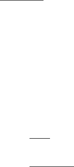
Figure 11.8 shows the discrete exponential distribution. We see from the figure

that a places the pmf at the desired position on the time axis, and x determines how

fast the exponential function decays with time. The distribution in (11.58) is a valid

pmf since its sum equals unity. The values of α and x will be derived in the next

section.

Example 11.10 Find the average value for the geometrically distributed interarrival

time given by (11.58).

Fig. 11.8 A biased geometric

distribution with two design

parameters: position

parameter α and packet

arrival probability x

p(N = n)

avg

Interarrival time

404 11 Modeling Network Traffic

The average number of time steps between packets n

is given by

∞



n=α

nx(1 − x)

n−α

+α

We see that as the probability for packet arrival decreases (x  1), the average

number of steps between packets increases as expected. A high value for α implies

slow traffic since the minimum separation between packets is large. This results in

increased values for n

The expression we obtained for the average interarrival time reduces to the ex-

pression obtained in Example 11.8 for the simple exponential distribution when the

position parameter α → 0.

11.4.4 Extracting Bernoulli Traffic Parameters

In this section, we show how to find the values of the position parameter a and

packet arrival probability x for a source whose average rate ␭

and burst rate σ are

known.

The position parameter α in (11.58) is found by studying packet arrival during

a period t. The time step T associated with this discrete arrival process is arbitrary

and depends on the specifics of the system being studied.

If we study our system for a time period t, then the number of time steps n

spanned by this time period is given by

n =

(11.59)

The maximum number of packets N

that could arrive during this time period

depends on the burst rate σ

= σ × t (11.60)

where σ was assumed to be given in units of packets/second.

The minimum number of time steps between adjacent packets when the source

is transmitting packets at the burst rate is given by

α =

)

σ T

(11.61)

where the floor function is used to find a conservative estimate of α.Nowwehave

an expression for the position parameter a for the biased exponential distribution

that depends on the source burst rate and the time step value.

11.4 Discrete-Time Modeling: Interarrival Time for Bernoulli Traffic 405

Now we turn our attention to estimating the arrival probability x. Consider a

time period t again, which corresponds to n time steps. Because we have Bernoulli

traffic, we can estimate x from the average number of packets received in that time

period t which corresponds to n time steps:

= x × n (11.62)

The average number of packets can also be estimated from the average data

rate ␭

= λ

×t (11.63)

We can find a value of x from the above two equations as

x =

×t

= λ

T (11.64)

Example 11.11 An ATM data source follows the binomial distribution and has an

average data rate of ␭

= 400 packets/s and maximum burst rate of σ = 10

pack-

ets/s. Estimate the geometric distribution parameters that best describe that source

if the time step value T chosen is equal to 0.1 ms.

The position parameter is given by

α = 10 time steps

and the packet arrival probability per time step is given by

x = 0.04

Thus the pmf describing the interarrival time is given by

p(N = n) = 0.04 ×0.96

n−10

11.4.5 Bernoulli Traffic and Queuing Analysis

The previous subsection discussed how the biased geometric distribution parameters

can be extracted given the system parameters:

␭

the average data rate

σ the maximum data rate expected from the source

A Bernoulli source matching these given parameters has position and shape

parameters:

406 11 Modeling Network Traffic

a = 1/(σ T ) (11.65)

x = λ

T (11.66)

In this section, we ask the question: Given a Bernoulli source with known param-

eters that feeds into a queue, what is the packet arrival probability for the queue?

Remember that in queuing theory the two most important descriptors are the arrival

statistics and the departure statistics. The analysis we undertake is very similar to

the one done for Poisson traffic in Section 11.4.

There are two cases that must be studied separately based on the values of the

step size T and the position parameter a.

Case When T ≤ a

The case T ≤ a implies that we are sampling our queue at a very high rate that is

greater than the burst rate of the source. Therefore, when T ≤ a at most, one packet

could arrive in one time step with probability x that we have to determine.

The number of time steps over a time period t is estimated as

n =

(11.67)

The average number of packets arriving over a period t is given by

= λ

nT (11.68)

From the binomial distribution, the average number of packets in one step time is

= xn (11.69)

where x is the packet arrival probability in one time step.

From the above two equations, the packet arrival probability per time step is

given by

x = λ

T (11.70)

We see in the above equation that as T gets smaller or as the source activity is

reduced (small λ

), the arrival probability is decreased, which makes sense.

Case When T > a

The case T > a implies that we are sampling our queue at a rate that is slower than

the burst rate of the source. Therefore, when T > a, more than one packet could

arrive in one time step and we have to find the packet arrival statistics that describe

this situation.

11.5 Self-Similar Traffic 407

We start our estimation of the arrival probability x by determine the maximum

number of packets that could arrive in one step time

=σ T  (11.71)

The ceiling function was used here after assuming that the receiver will consider

packets that partly arrived during one time step. If the receiver does not wait for

partially arrived packets, then the floor function should be used.

The average number of packets arriving in the time period T is

(in) = λ

T (11.72)

From the binomial distribution, the average number of packets in one step time is

(in) = xN

(11.73)

From the above two equations, the packet arrival probability per time step is

x =

(11.74)

The probability that k packets arrive at one time step T is given by the binomial

distribution

p(k) =





(1 − x)

−k

(11.75)

11.5 Self-Similar Traffic

We are familiar with the concept of periodic waveforms. A periodic signal repeats

itself with additive translations of time. For example, the sine wave sin ωt will have

the same value if we add an integer, multiple of the period T = 2π/ω since

sin ωt = sin ω(t +i T )

On the other hand, a self-similar signal repeats itself with multiplicative changes

in the time scale [13, 14]. Thus a self-similar waveform will have the same shape

if we scale the time axis up or down. In other words, imagine we observe a certain

waveform on a scope when the scope is set at 1 ms/division. We increase the res-

olution and set the scale to 1␮s/division. If the incoming signal is self-similar, the

scope would display the same waveform we saw earlier at a coarser scale.

Self-similar traffic describes traffic on Ethernet LANs and variable-bit-rate video

services [2–7]. These results were based on analysis of millions of observed packets

over an Ethernet LAN and an analysis of millions of observed frame data generated

408 11 Modeling Network Traffic

by variable-bit-rate (VBR) video. The main characteristic of self-similar traffic is

the presence of “similarly-looking” bursts at every time scale (seconds, minutes,

hours) [12].

The effect of self-similarity is to introduce long-range (large-lag) autocorrelation

into the traffic stream, which is observed in practice. This phenomenon leads to

periods of high traffic volumes even when the average traffic intensity is low. A

switch or router accepting self-similar traffic will find that its buffers will be over-

whelmed at certain times even if the expected traffic rate is low. Thus switches with

buffer sizes, selected based on simulations using Poisson, traffic, will encounter un-

expected buffer overflow and packet loss. Poisson traffic models predict exponential

decrease in data loss as the buffer size increases since the probability of finding the

queue in a high-occupancy state decreases exponentially. Self-similar models, on the

other hand, predict stretched exponential loss curves. This is why increasing link

capacity is much more effective in improving performance than increasing buffer

size. The rational being that it is better to move the data along than to attempt to

store them since any buffer size selected might not be enough when self-similar

traffic is encountered.

11.6 Self-Similarity and Random Processes

Assume that we have a discrete-time random process X(n) that produces the set of

random variables

{

, X

, ···

}

. We define the aggregated random process X

as a

random process whose data samples are calculated as

(m)



+ X

+···+X

m−1



(m)



+ X

m+1

+···+X

2m−1



(m)



+ X

2m+1

+···+X

3m−1



The random process is self-similar if it satisfies the following properties.

1. The processes X and X

(m)

are related by the equation

(m)

(1−H)

X (11.76)

where H is the Hurst parameter (0.5 < H < 1).

2. The means of X and X

(m)

are equal

E[X] = E[X

(m)

] = μ (11.77)