Gebali F. Analysis Of Computer And Communication Networks
Подождите немного. Документ загружается.

10.7 IEEE 802.11: DCF Function for Ad Hoc Wireless LANs 359
0 16
10
–4
10
–3
10
–2
10
–1
10
0
32
Input traffic
Access Probability
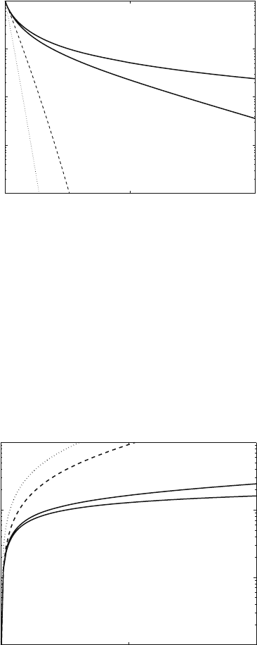
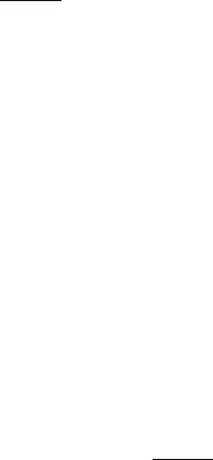
Fig. 10.23 Access probability for the IEEE 802.11 protocol versus the average input traffic when
w = 8, n = 10, and N = 32. The upper solid line is the access probability of IEEE 802.11/DCF,
the lower solid line is the access probability of CSMA/CA, the dashed line represents the ac-
cess probability of slotted ALOHA, and the dotted line represents the access probability of pure
ALOHA
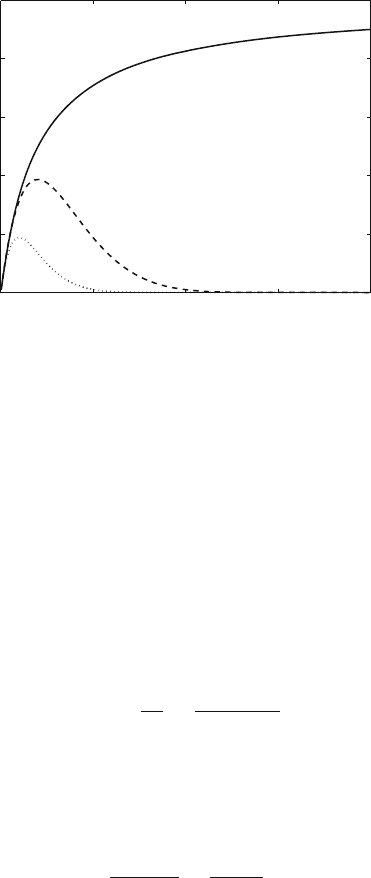
Figure 10.24 shows the energy of IEEE 802.11/DCF when w = 8, n = 10, and
N = 32. The lower solid line is the energy of IEEE 802.11/DCF, the upper solid
line is the energy of CSMA/CA, the dashed line represents the energy of slotted
ALOHA, and the dotted line represents the energy of pure ALOHA.
0
10
–1
10
0
10
1
10
2
16 32
Input traffic
Energy (dB)
Fig. 10.24 Energy for the IEEE 802.11/DCF protocol versus the average input traffic when w = 8,
n = 10, and N = 32. The lower solid line is the energy of IEEE 802.11/DCF, the upper solid line is
the energy of CSMA/CA, the dashed line represents the energy of slotted ALOHA, and the dotted
line represents the energy of pure ALOHA
360 10 Modeling Medium Access Control Protocols
0
10
–1
10
0
10
1
10
2
10
3
10
4
10
5
16 32
Input traffic
Delay
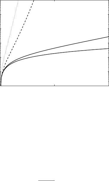
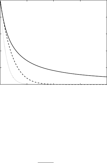
Fig. 10.25 Delay for the IEEE 802.11/DCF protocol versus the average input traffic when w = 8,
n = 10, and N = 32. The lower solid line is the delay of IEEE 802.11/DCF, the upper solid line
is the delay of CSMA/CA, the dashed line represents the delay of slotted ALOHA, and the dotted
line represents the delay of pure ALOHA
The average number of attempts for a successful transmission is
n
a
=
∞
i=0
i (1 − p
a
)
i
p
a
=
1 − p
a
p
a
(10.103)
Figure 10.25 shows the delay of IEEE 802.11/DCF when w = 8, n = 10, and
N = 32. The lower solid line is the delay of IEEE 802.11/DCF, the upper solid line
is the delay of CSMA/CA, the dashed line represents the delay of slotted ALOHA,
and the dotted line represents the delay of pure ALOHA.
10.7.4 IEEE 802.11/DCF Final Remarks
The DCF mode of the IEEE 802.11 protocols has been studied by many researchers.
We tried to present here a simple model to start the reader in the area of model-
ing protocols. However, there are many ripe areas that have not been adequately
explored for this protocol and for others also. We enumerate some of these direc-
tions:
1. Channel errors have not been considered. This is a physical layer problem but
could also be considered in a cross-layer modeling. What matters here is to obtain
the probability that a frame or packet is in error.
10.8 IEEE 802.11: PCF Function for Infrastructure Wireless LANs 361
2. Simple backoff strategies were used here in order to obtain simple expressions.
Adopting binary exponential backoff (BEB) strategy would result in a model that
requires an iterative solution.
3. Perhaps the most serious deficiency in the models in this chapter is the implicit
assumption that no new traffic arrives while the user is attempting to access the
channel. This amounts to assuming the transmit buffer has a single storage lo-
cation only. Using a more realistic buffer would require solving two queuing
systems.
10.8 IEEE 802.11: PCF Function for Infrastructure Wireless
LANs
In the IEEE 802.11, there is a feature to support quality of service (QoS) in infras-
tructure LANs through implementation of the point coordination function (PCF). A
central controller polls the users to determine which user can access the medium
in the next frame. Such medium access scheme is used in infrastructure wireless
LANs where a central controller is provided to coordinate the activities of the users
or mobile terminals. The central controller in wireless LANs such as HiperLAN/2
is called the access point (AP).
The central controller prevents collisions from taking place since it coordi-
nates access to the channel through implementation of some kind of reservation or
scheduling algorithm. Thus we can classify the IEEE 802.11/PCF as a reservation-
based scheme that is collision-free.
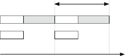
In IEEE 802.11, using the PCF function, time is divided into time steps as shown
in Fig. 10.26. There are two directions of communication: the uplink from the users
to the central controller and downlink from the central controller to the users. The
uplink frames consist of a request phase and a data phase. In the request phase, users
issue their requests and in the data phase, users send their data when they are told to
do so by the central controller or scheduler.
time
Requests
Scheduling
Data packet Requests
Scheduling
Data packet
Uplink
Downlink
One frame
Fig. 10.26 Frame structure for IEEE 802.11 protocol using the PCF function
362 10 Modeling Medium Access Control Protocols
The data phase transmits one frame in the uplink direction from one user based
on some scheduling policy. The receiver is told by the central controller to expect
an arriving frame. Alternatively, all users receive the transmitted frame and decide
whether it was destined to them or not.
IEEE 802.11/PCF is efficient when the time taken by the request phase is much
smaller than the data phase if both the uplink and downlink use the same channel.
If there are two separate channels, then the protocol is efficient as long as the delay
of the request phase is smaller than the duration of the data phase. If the central
controller requires a time that is comparable to the data phase, then the channel is
not well used and other MAC techniques should be used.
10.8.1 IEEE 802.11: PCF Medium Access Control
The central controller communicates with the users through the downlink. The con-
troller polls all users in the system and schedules only one user to access the medium
based on some scheduling strategy. In addition, the controller informs the receivers
to be ready for the transmitted frames. In a nonpersistent PCF protocol, users that
were not granted access to the channel issue another request to transmit with prob-
ability p when polled by the access point on the next poll period. A large value for
the persistence probability p would ensure that the user gets to compete in the next
poll period. On the other hand, a small p reduces the number of contending users.
We propose here to adopt a variable or adaptive persistence strategy. A user with
heavy traffic would use a large value for p, while a user with low traffic would use
a small value for p.
10.8.2 IEEE 802.11: Nonpersistent PCF Model Assumptions
In this section, we perform Markov chain analysis of the IEEE 802.11 (PCF) proto-
col. We make the following assumptions for our analysis of the simple
protocol:
1. The states of the Markov chain represent the channel state which could be idle
or transmitting.
2. The time step is equal to the poll period of the central controller.
3. The system has a fixed population of N users.
4. There is a single customer class. The case of multiple customer classes is treated
in Problem 10.46.
5. All frames have equal lengths and each frame requires n time steps to be trans-
mitted.
6. Probability that a user requests transmission during a time step is a and proba-
bility that the user is idle during a time step is b = 1 −a.
10.8 IEEE 802.11: PCF Function for Infrastructure Wireless LANs 363
y
x
Idle
Transmitting
i
t
1
1
1
1
...
1
t
2
t
n
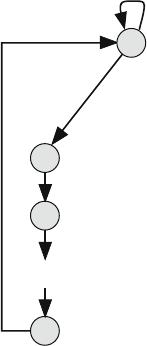
Fig. 10.27 State transition diagram for the channel of the IEEE 802.11 protocol employing the
PCF function
7. If a user is refused access to the channel, it will issue a request at the next
poll period with persistence probability equal to the frame arrival probability
(i.e., p = a).
8. The channel is assumed to be always available for transmission in every time
step.
The state diagram for the channel is shown in Fig. 10.27. In the figure, x is the
probability that all users are idle and do not issue a request to access the channel
during the current time step and y = 1 − x. No collision takes place when more
than one request is present due to polling. The controller will then decide which
station is granted access and inform the others of that decision through ACK/NAK
mechanism. We can write
x = b
N
(10.104)
We organize the distribution vector at equilibrium as follows:
s =
s
i
s
t
1
s
t
2
··· s
t
n
t
(10.105)
where s
i
is the idle state and s
t
j
is the state when the channel is transmitting the jth
part of the frame. The corresponding transition matrix of the channel is given by
364 10 Modeling Medium Access Control Protocols
P =
⎡
⎢
⎢
⎢
⎢
⎢
⎣
x 00··· 1
y 00··· 0
010··· 0
.
.
.
.
.
.
.
.
.
.
.
.
.
.
.
000··· 0
⎤
⎥
⎥
⎥
⎥
⎥
⎦
(10.106)
At equilibrium, the distribution vector is obtained by solving the two equations
Ps = s (10.107)
s
i
+
i=1
t
i
= 1 (10.108)
From the structure of the matrix, we can write
t
1
= t
2
=···=t
n
= t (10.109)
We also have
t = ys
i
(10.110)
Using simple algebra, we can finally obtain the distribution vector as
s =
1
ny +1
1 y ··· y
t
(10.111)
10.8.3 IEEE 802.11: Nonpersistent PCF Protocol Performance
Having obtained the transition matrix, we are able to find the performance of the
nonpersistent IEEE 802.11/PCF channel.
The input traffic is defined here as the average number of requests per time step
and is given by
N
a
(in) =
N
i=0
i
N
i
a
i
(1 −a)
N−i
= Na (10.112)
The throughput of the system is given by
Th =
i=1
ns
t
i
=
ny
ny +1
(10.113)
Notice that when n →∞, the maximum throughput approaches 1. This is
because comparatively little time is wasted polling the users. On the other hand,
10.8 IEEE 802.11: PCF Function for Infrastructure Wireless LANs 365
0 2.5 5 7.5 10
0
0.2
0.4
0.6
0.8
1
Input traffic
Throughput
Fig. 10.28 The throughput for nonpersistent IEEE 802.11/PCF versus the average input traffic
when n = 50 and N = 10. The solid line is the throughput of nonpersistent IEEE 802.11/PCF,
the dashed line represents the throughput of slotted ALOHA, and the dotted line represents the
throughput of pure ALOHA
when n ≈ 1, the maximum throughput approaches 50%. This is because approxi-
mately 50% of the time the access point is polling the users and no frames are being
transmitted during the period.
Figure 10.28 shows the throughput of the nonpersistent IEEE 802.11/PCF pro-
tocol when n = 50 and N = 10. The solid line is the throughput of nonpersistent
IEEE 802.11/PCF, the dashed line represents the throughput of slotted ALOHA, and
the dotted line represents the throughput of pure ALOHA.
Because all users are the same, the throughput seen by one user is given by
Th(user) =
Th
N
=
ny
N(ny +1)
(10.114)
When n is very large, the maximum throughput for each user will approach 1/N.
This is to be expected due to the fair sharing of the medium among the users.
Define p
a
as the access probability for one user which is given by
p
a
=
Th(user)
a
=
Th
N
a
(in)
(10.115)
Figure 10.29 shows the access probability of nonpersistent IEEE 802.11/PCF
when n = 50 and N = 10. The solid line is the access probability of nonpersis-
tent IEEE 802.11/PCF, the dashed line represents the access probability of slotted
ALOHA, and the dotted line represents the access probability of pure ALOHA.
Having found the acceptance probability, we are able to determine the average
number of attempts before a user gets access to the medium:
366 10 Modeling Medium Access Control Protocols
0 2.5 5 7.5 10
0
0.2
0.4
0.6
0.8
1
Input traffic
Acceptance Probability
Fig. 10.29 Delay for the nonpersistent IEEE 802.11 protocol versus the average input traffic per
time step when n = 50 and N = 10. The solid line is the access probability of IEEE 802.11/PCF,
the dashed line represents the access probability of slotted ALOHA, and the dotted line represents
the access probability of pure ALOHA
n
a
=
∞
k=0
k
(
1 − p
a
)
k
p
a
(10.116)
=
1 − p
a
p
a
(10.117)
Figure 10.30 shows the delay of nonpersistent IEEE 802.11/PCF when n = 50
and N = 10. The solid line is the delay of nonpersistent IEEE 802.11, the dashed
line represents the delay of slotted ALOHA, and the dotted line represents the delay
of pure ALOHA.
10.8.4 IEEE 802.11: 1-Persistent PCF
This section deals with modeling the point coordination function (PCF) of the
1-persistent IEEE 802.11 protocol. We make the following assumptions for our
analysis of the simple protocol.
1. The states of the Markov chain represent the number of queued users requesting
access to the channel at the start of any time step.
2. Time is divided into time steps such that each time step starts with a control phase
and then a data phase. In the control phase, all arriving requests are processed
and one access is granted. In the data phase, the user that was granted access to
the medium transfers its data.
3. The system has a fixed population of N users.
10.8 IEEE 802.11: PCF Function for Infrastructure Wireless LANs 367
0 2.5
10
–2
10
0
10
2
10
4
5 7.5 10
Input traffic
Delay
Fig. 10.30 Delay for the nonpersistent IEEE 802.11/PCF protocol versus the average input traf-
fic per time step when n = 50 and N = 10. The solid line is the delay of nonpersistent IEEE
802.11/PCF, the dashed line represents the delay of slotted ALOHA, and the dotted line represents
the delay of pure ALOHA
4. There is a single customer class. The case of multiple customer classes is treated
in Problem 10.46.
5. A user can have, at most, one message waiting for transmission. At the end of
certain time step, users that have requests pending cannot issue more requests at
the next time step.
6. A user that is transmitting at a certain time step can issue a new request at the
next time step.
7. Users that were denied access will attempt a retransmission at the next time step.
8. Probability that a user requests transmission is a and probability that the user is
idle is b = 1 −a.
9. The channel is assumed to be always available for transmission in every time
step.
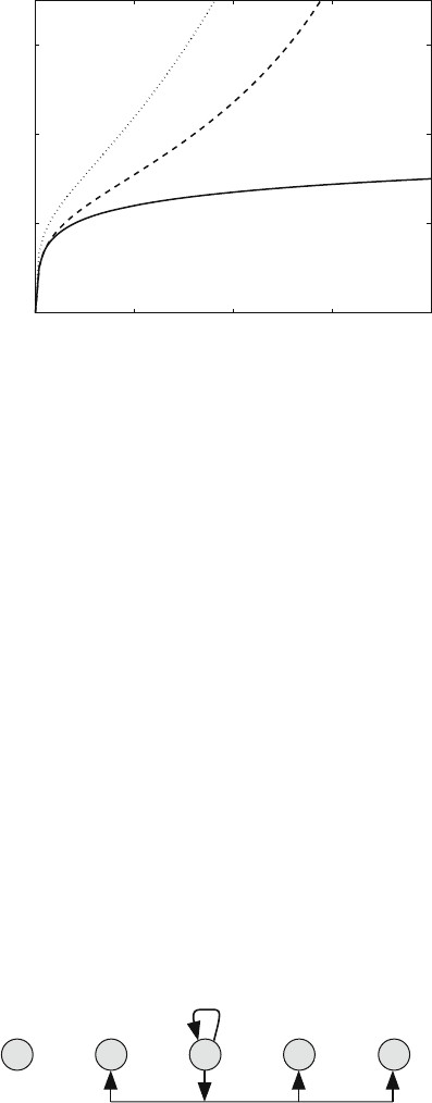
The state diagram for the system is shown in Fig. 10.31 where the user popu-
lation is N. Only transitions out of state 2 are shown for simplicity. In the figure,
state i indicates that there are i users requesting transmission. Based on the above
assumptions, it is impossible for the system to have N queued requests since one
request is always guaranteed to be processed in the same time step. The request
2301
4
N
4
Fig. 10.31 State transition diagram for the single access reservation-based MAC protocol when
the system has N = 5 users. Only transitions out of state 2 are shown for simplicity
368 10 Modeling Medium Access Control Protocols
queue will vary in size between the limits 0 and N − 1 since at worst N requests
could arrive at a time step but only N −1 requests will remain queued at the end of
the time step.
Starting at state j, the probability of making a transition to state i is governed by
the following observations:
• It is impossible to make a transition to state i if i < j −1 since only one user can
access the medium.
• Itispossibletostayinthesamestate j when one user leaves the system and
exactly one more user requests access.
• The next state would be in the range j ≤ i < N depending on how many users
request access to the medium.
• The transition probability p
ij
represents the probability that i users still request
access to the medium at the end of the current time step.
According to the assumptions we employed, the resulting transition matrix is
lower N × N Hessenberg matrix in which all the element p
ij
= 0for j > i + 1.
Suppose there are j queued requests at the end of a time step. In the next time step,
we are sure that j requests will be issued plus a possible 0 to N − j additional
requests coming from the other users.
We organize the distribution vector at equilibrium as follows:
s =
s
0
s
1
s
2
··· s
N−1
t
(10.118)
where s
i
corresponds to the system state when there are i users with unsatisfied
(queued) requests. The corresponding transition matrix of the channel is given by
P =
⎡
⎢
⎢
⎢
⎢
⎢
⎢
⎢
⎢
⎢
⎢
⎢
⎣
yp(N −1, 0) ··· 00
p(N, 2) p(N − 1, 1) ··· 00
p(N, 3) p(N − 1, 2) ··· 00
p(3, 4) p(N −1, 3) ··· 00
.
.
.
.
.
.
.
.
.
.
.
.
.
.
.
p(N, N −2) p(N −1, N −3) ··· p(2, 0) 0
p(N
, N −1) p(N −1, N −2) ··· p(2, 1) p(1, 0)
p(N, N) p(N −1, N −1) ··· p(2, 2) p(1, 1)
⎤
⎥
⎥
⎥
⎥
⎥
⎥
⎥
⎥
⎥
⎥
⎥
⎦
(10.119)
where p(i, j) is the probability that there were i idle users and j of them issued
requests to access the medium. y represents the probability that there were N idle
users and at most one of them issued a request:
p(i, j) =
i
j
a
i−j
b
j
(10.120)
y = p(N, 0) + p(N, 1) (10.121)