Gebali F. Analysis Of Computer And Communication Networks
Подождите немного. Документ загружается.


238 7 Queuing Analysis
From (7.30), the transition matrix is
P =
⎡
⎢
⎢
⎢
⎢
⎢
⎢
⎢
⎢
⎢
⎣
0.88 0.320000···
0.12 0.56 0.32000···
00.12 0.56 0.32 0 0 ···
000.12 0.56 0.32 0 ···
0000.12 0.56 0.32 ···
00000.12 0.56 ···
.
.
.
.
.
.
.
.
.
.
.
.
.
.
.
.
.
.
.
.
.
⎤
⎥
⎥
⎥
⎥
⎥
⎥
⎥
⎥
⎥
⎦
The steady-state distribution vector is found using (7.37)
s =
0.6297 0.2361 0.0885 0.0332 0.0125
t
Compare this distribution vector with the distribution vector of Example 7.1,
which described an infinite-sized queue with the same arrival and departure statis-
tics. We see that components of the distribution vector here are slightly larger than
their counterparts in the infinite-sized queue as expected.
The queue performance is as follows:
N
a
(out) = Th = 0.5985 packets/time step
η = 0.9975
N
a
(lost) = 1.5 ×10
−3
packets/time step
L = 0.0025
Q
a
= 0.5626 packets
W = 0.9401 time steps
We note that the M/M/1/B queue has smaller average size Q
a
and smaller
wait time W compared to the M/M/1 queue with the same arrival and departure
statistics. As expected, we have
N
a
(out) + N
a
(lost) = N
a
(in)
Example 7.4 Find the performance of the queue in the previous example when the
queue size becomes B = 20.
The queue performance is as follows:
N
a
(out) = Th = 0.6 packets/time step
η = 1
N
a
(lost) = 2.2682 ×10
−10
packets/time step
L = 3.7804 ×10
−10
Q
a
= 0.6 packets
W = 1 time steps
7.6 M/M/1/B Queue 239
We see that increasing the queue size exponentially decreases the loss probability.
The throughput is not changed by much, but the wait time is slightly increased due
to the increased average queue size.
Example 7.5 Plot the M/M/1/B performance when the input traffic varies between
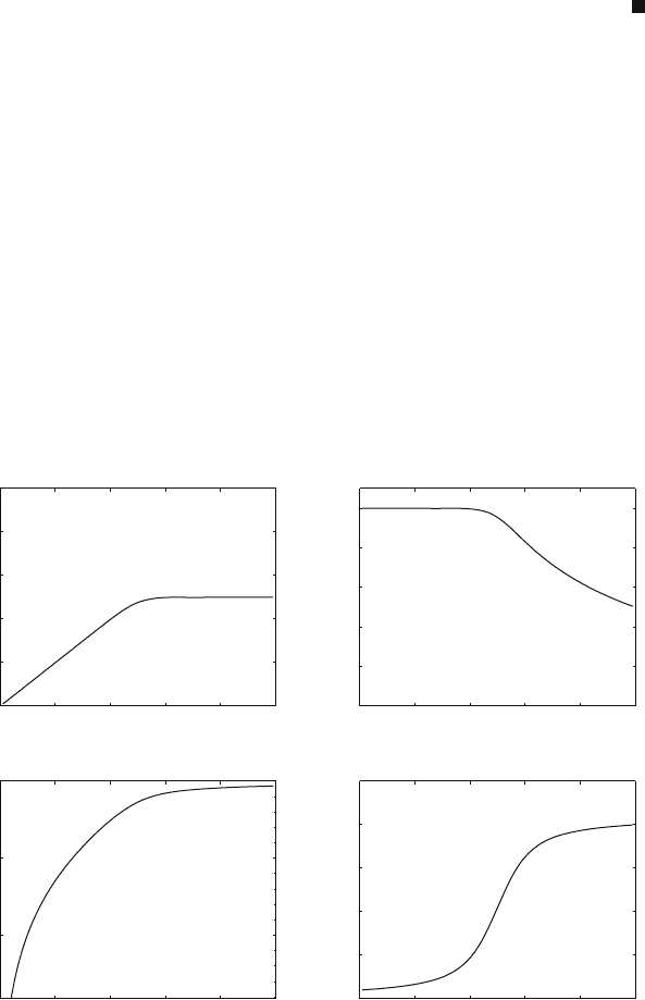
0 ≤ a ≤ 1forB = 10 and c = 0.5.
Figure 7.5 shows the throughput, efficiency, loss probability, and delay to plot
these quantities versus input traffic.
The important things to note from this example are as follows:
1. The throughput of the queue could not exceed the maximum value for the av-
erage output traffic. Section 7.6.2 below will prove that this maximum value is
simply c.
2. The efficiency of the queue is very close to 100% until the input traffic
approaches the maximum output traffic c.
3. Packet loss probability is always present but starts to increase when the input
traffic approaches the packet maximum output traffic c.
4. Packet delay increases sharply when the input traffic approaches the packet max-
imum output traffic c.
0 0.2 0.4 0.6 0.8 1
0 0.2 0.4 0.6 0.8 1
0
0.2
0.4
0.6
0.8
1
0 0.2 0.4 0.6 0.8 1
0 0.2 0.4 0.6 0.8 1
0
0.2
0.4
0.6
0.8
1
Input traffic
Throughput
Input traffic
Efficiency
10
−10
10
−5
100
Input traffic
Loss probability
0
5
10
15
20
25
Input traffic
Delay
Fig. 7.5 M/M/1/B throughput, efficiency, loss probability, and delay to plot versus input traffic
when B = 10 and c = 0.5

240 7 Queuing Analysis
5. Congestion conditions occur as soon as the input traffic exceeds the maximum
output traffic c. Congestion is characterized by decreased efficiency, increased
packet loss, and increased delay.
6. The delay reaches a maximum value determined by the maximum size of the
queue and the maximum output traffic c. The maximum delay could be approxi-
mated as
Maximum Delay =
B
c
= 20 time steps
7.6.2 Performance Bounds on M/M/1/B Queue
The previous example helped us get some rough estimates for the performance
bounds of the M/M/1/B queue. This section formalizes these estimates.
Under full load conditions, the M/M/1/B become full and we can assume
a → 1 (7.51)
b → 0 (7.52)
s
0
→ 0 (7.53)
s
B
→ 1 (7.54)
Q
a
→ B (7.55)
The maximum throughput is given from (7.39) by
Th(max) = N
a
(out)
max
= c (7.56)
The departure probability is most important for determining the maximum
throughput of the queue.
The minimum efficiency of the queue is given from (7.42) by
η(min) = c (7.57)
The departure probability is most important for determining the efficiency of the
queue.
The maximum lost traffic is given from (7.43) by
N
a
(lost)
max
= d = 1 −c (7.58)
The maximum packet loss probability is given from (7.45) by
L(max) = 1 −c (7.59)

7.7 M
m
/M/1/B Queue 241
The maximum wait time is given by the approximate formula
W(max) =
B
c
(7.60)
Larger queues result in larger wait times as expected.
7.7 M
m
/M/1/B Queue
In an M
m
/M/1 queue at any time step, at most m customers could arrive and at
most one customer could leave. We shall encounter this type of queue when we
study network switches where first-in-first-out (FIFO) queues exist at each output
port. For each queue, a maximum of m packets arrive at the queue input but only
one packet can leave the queue. Therefore, the queue size can increase by more
than one, but can only decrease by one in each time step. Assume that the binomial
probability of k arrivals at instant n is given by
a
k
=
m
k
a
k
b
m−k
(7.61)
where a is the probability that a packet arrives, b = 1 −a, and m is the maximum
number of packets that could arrive at the queue input. The queue size can only
decrease by at most one at any instant with probability c. The probability that no
packet leaves the queue is d = 1−c. We assume that when a packet arrives, it could
be serviced at the same time step and it could leave the queue with probability c.
The condition for the stability of the queue is
m
k=0
ka
k
= am< c (7.62)
which indicates that the average number of arrivals at a given time is less than the
average number of departures from the system. The resulting state transition matrix
is a lower (B + 1) × (B + 1) Hessenberg matrix in which all the elements p
ij
= 0
for j > i +1:
P =
⎡
⎢
⎢
⎢
⎢
⎢
⎢
⎢
⎣
xy
0
0 ··· 00
y
2
y
1
y
0
... 00
y
3
y
2
y
1
··· 00
.
.
.
.
.
.
.
.
.
.
.
.
.
.
.
.
.
.
y
B
y
B−1
y
B−2
··· y
1
y
0
z
B
z
B−1
z
B−2
··· z
1
z
0
⎤
⎥
⎥
⎥
⎥
⎥
⎥
⎥
⎦
(7.63)

242 7 Queuing Analysis
where
x = a
1
c +a
0
(7.64)
y
i
= a
i
c +a
i−1
d (7.65)
z
i
= a
i
d +
m
k=i+1
a
k
(7.66)
whereweassumed
a
k
= 0 k < 0 (7.67)
a
k
= 0 k > m (7.68)
The above transition matrix has m subdiagonals when m ≤ B.
7.7.1 M
m
/M/1/B Queue Performance
To calculate the throughput of the M
m
/M/1/B, we need to consider the queue in
two situations: when it is empty and when it is not.
The throughput of the M
m
/M/1/B queue when the queue is in state s
0
is
given by
Th
0
= (1 −a
0
) c (7.69)
This is simply the probability that one or more packets arrive and one packet
leaves the queue. When the queue is in any other state, the throughput is given by
Th
i
= c 1 ≤ i ≤ B (7.70)
This is simply the probability that a packet leaves the queue. The average
throughput is estimated as
Th =
B
i=0
Th
i
s
i
= c
(
1 −a
0
s
0
)
(7.71)
The throughput is measured in units of packets/time step. The throughput in units
of packets/s is
Th
=
Th
T
(7.72)
7.7 M
m
/M/1/B Queue 243
The input traffic is given by
N
a
(in) =
m
i=0
ia
i
= ma (7.73)
The efficiency of the M
m
/M/1/B queue is given by
η =
N
a
(out)
N
a
(in)
=
Th
ma
=
c
(
1 −a
0
s
0
)
ma
(7.74)
Data are lost in the M
m
/M/1/B queue when it becomes full and packets arrive
but does not leave. However, due to multiple arrivals, packets could be lost even
when the queue is not completely full. For example, we could still have one location
left in the queue but three customers arrive. Definitely packets will be lost then.
Therefore, we conclude that average lost traffic N
a
(lost) is a bit difficult to obtain.
However, the traffic conservation principle is useful in getting a simple expression
for lost traffic. The average lost traffic N
a
(lost) is given by
N
a
(lost) = N
a
(in) − N
a
(out)
= ma−c
(
1 −a
0
s
0
)
(7.75)
The lost traffic is measured in units of packets per time step. The average lost
traffic measured in packets per second is given by
N
a
(lost) =
N
a
(lost)
T
(7.76)
The packet loss probability L is the ratio of lost traffic relative to the input traffic:
L =
N
a
(lost)
N
a
(in)
= 1 −η
= 1 −
c
(
1 −a
0
s
0
)
ma
(7.77)
The average queue size is given by the equation
Q
a
=
B
i=0
is
i
(7.78)

244 7 Queuing Analysis
We can invoke Little’s result to estimate the wait time, which is the average num-
ber of time steps a packet spends in the queue before it is routed, as
Q
a
= W ×Th (7.79)
where W is the average number of time steps that a packet spends in the queue.
Thus, W is given by
W =
Q
a
Th
(7.80)
The wait time is measured in units of time steps. The wait time in units of seconds
is given by the unnormalized version of Little’s result:
W
=
Q
a
Th
(7.81)
Example 7.6 Consider the M
m
/M/1/B queue with the following parameters
a = 0.04, m = 2, c = 0.1, and B = 5. Check its stability condition and find
the equilibrium distribution vector and queue performance.
The packet arrival probability is
a
k
=
2
k
(0.04)
k
(0.96)
2−k
The stability condition is found from (7.62):
2
k=0
ka
k
= 0.08 < c
The queue is stable and the transition matrix is
P =
⎡
⎢
⎢
⎢
⎢
⎢
⎢
⎣
0.9293 0.0922 0000
0.0693 0.8371 0.0922 0 0 0
0.0014 0.0693 0.8371 0.0922 0 0
00.0014 0.0693 0.8371 0.0922 0
000.0014 0.0693 0.8371 0.0922
0000.0014 0.0707 0.9078
⎤
⎥
⎥
⎥
⎥
⎥
⎥
⎦
The transition matrix has two subdiagonals because m = 2.
The steady-state distribution vector is the eigenvector of P that corresponds to
unity eigenvalue. We have
s =
0.2843 0.2182 0.1719 0.1353 0.1065 0.0838
t

7.7 M
m
/M/1/B Queue 245
We see that the most probable state for the queue is state s
0
which occurs with
probability 28.43%.
The queue performance is as follows:
Th = 0.0738 packets/time step
η = 0.9225
N
a
(lost) = 6.2 ×10
−3
packets/time step
L = 0.0775
Q
a
= 1.813 packets
W = 24.5673 time steps
Flow conservation is verified since the sum of the throughput and the lost traffic
equals the input traffic N
a
(in) = ma.
Example 7.7 Find the performance of the queue in the previous example when the
queue size becomes B = 20. The queue performance is as follows:
Th = 0.0799 packets/time step
η = 0.9984
N
a
(lost) = 1.3167 ×10
−4
packets/time step
L = 0.0016
Q
a
= 1.813 packets
W = 44.3432 time steps
We see that increasing the queue size decreases the loss probability which results
in only a slight increase in the throughput. The wait time is almost doubled.
In Chapter 4, we explored different techniques for finding the equilibrium dis-
tribution for the distribution vector s. For simple situations when the value of m is
small (1 or 2), we can use the difference equation approach. When m is large, we
can use the z-transform technique as in Section 4.8.
Example 7.8 Plot the M
m
/M/1/B performance when m = 2 and the input traffic
varies between 0 ≤ a ≤ 1forB = 10 and c = 0.5.
Figure 7.6 shows the variation of the throughput, efficiency, loss probability, and
delay versus the average input traffic.
The important things to note from this example are as follows:
1. The throughput of the queue could not exceed the maximum output traffic c.
2. The efficiency of the queue is very close to 100% until the input traffic
approaches the maximum output traffic c.
3. Packet loss probability is always present but starts to increase when the input
traffic approaches the packet maximum output traffic c.
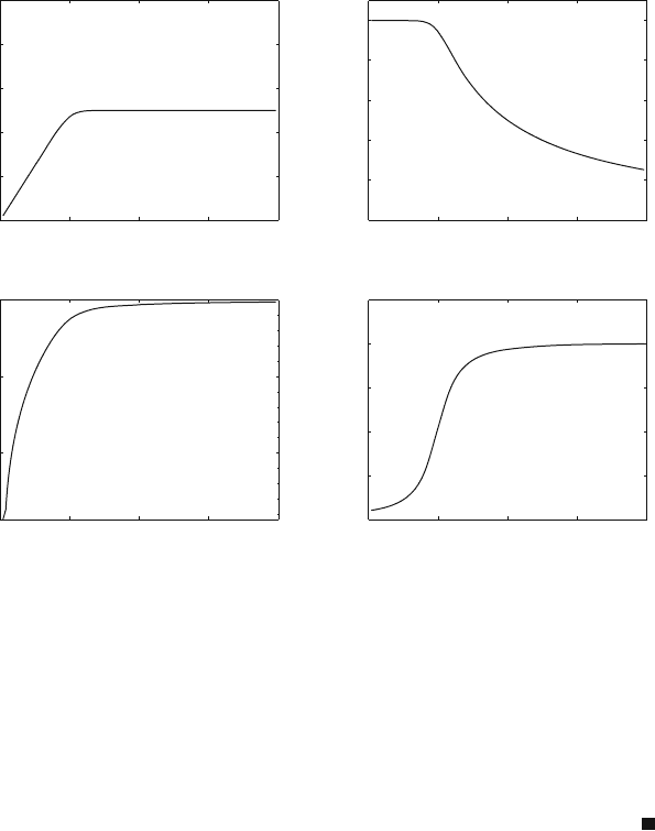
246 7 Queuing Analysis
0 0.5 1 1.5 2
0 0.5 1 1.5 2 0 0.5 1 1.5 2
0 0.5 1 1.5 2
0
0.2
0.4
0.6
0.8
1
0
0.2
0.4
0.6
0.8
1
Input traffic
Throughput
Input traffic
Efficiency
10
−10
10
−5
100
Input traffic
Loss probability
0
5
10
15
20
25
Input traffic
Delay
Fig. 7.6 M
m
/M/1/B throughput, efficiency, loss probability, and delay to plot versus input traffic
when m = 2, B = 10 and c = 0.5
4. Packet delay increases sharply when the input traffic approaches the packet max-
imum output traffic c.
5. Congestion conditions occur as soon as the input traffic exceeds the maximum
output traffic c. Congestion is characterized by decreased efficiency, increased
packet loss, and increased delay.
7.7.2 Performance Bounds on M
m
/M/1/B Queue
The previous example helped us get some rough estimates for the performance
bounds of the M
m
/M/1/B queue. This section formalizes these estimates.
Under full load conditions, the M
m
/M/1/B becomes full and we can assume
a → 1 (7.82)
b → 0 (7.83)
s
0
→ 0 (7.84)
s
B
→ 1 (7.85)
Q
a
→ B (7.86)

7.7 M
m
/M/1/B Queue 247
The maximum value for the throughput from (7.71) becomes
Th (max) = c (7.87)
The packet departure probability determines the maximum throughput of the
queue.
The minimum efficiency of the M
m
/M/1/B queue is given from (7.74) by
η(min) =
c
m
(7.88)
The maximum lost traffic is given from (7.77) by
N
a
(lost)
max
= m − c (7.89)
The maximum packet loss probability is given from (7.77) by
L(max) = 1 −
c
m
(7.90)
When more customers arrive per time step (large m), the probability of loss
increases. Maximum loss probability increases when packet departure probability
decreases and when the number of arriving customers increases.
The maximum delay is given from (7.80) by
W(max) =
B
Th(max)
=
B
c
(7.91)
7.7.3 Alternative Solution Method
When B is large, it is better to use numerical techniques such as forward- or back-
ward substitution using Givens rotations.
1
[5]
At steady state, we can write
Ps= s (7.92)
We can use the technique explained in Section 4.10 on page 140 to construct a
system of linear equations that can be solved using any of the specialized software
designed to solve large systems of linear equations.
1
Another useful technique for triangularizing a matrix is to use Householder transformation. How-
ever, we prefer Givens rotation due to its numerical stability. Alston Householder once commented
that he would never fly in an airplane that was designed with the help of a computer using floating
point arithmetic [4].