Gebali F. Analysis Of Computer And Communication Networks

Подождите немного. Документ загружается.

228 7 Queuing Analysis

of the famous M/M/1 queue for the continuous-time case. At a certain time step,

the probability of packet arrival is a, which is equivalent to a birth event or increase

in the queue population. The probability that a packet did not arrive is b = 1 − a.

The probability that a packet leaves the queue is c, which is equivalent to death or

reduction in the queue population. The probability that a packet does not leave the

queue is d = 1 − c. The probability c is representative of the server’s ability to

process the customers or packets in the queue in one time step.

The number of customers or packets stored in the queue is the state of our system.

Thus, the queue is in state s

when there are i customers or packets in the queue.

The state transition diagram for the discrete-time M/M/1 queue is shown in Fig. 7.1.

Changes in the queue size occur by at most one, i.e., only one packet could arrive or

depart. Thus, we expect the transition matrix to be tridiagonal.

The future state of the queue depends only on its current state. Thus, we can

model the queue as a discrete-time Markov chain. Since packet arrivals and de-

partures are independent of the time index value, we have a homogeneous Markov

chain. We assume that when a packet arrives, it could be serviced at the same time

step and it could leave the queue with probability c. This results in the transition

matrix given by

P =

⎡

⎢

⎣

bc 00···

ad f bc 0 ···

0 ad f bc ···

00ad f ···

⎤

⎥

⎦

(7.7)

where b = 1 −a, d = 1 −c, f

= 1 −ad, and f = ac +bd.

For example, starting with an empty queue (state s

), Fig. 7.1 indicates that we

move to state s

only when a packet arrives and no packet can depart, which is term

ad in the diagram. This transition is also indicated in the above transition matrix as

the term at location (2,1) of the transition matrix.

In order for the queue to be stable, the arrival probability must be smaller than

the departure probability (a < c).

Since the dimension of P is infinite, we are going to obtain an expression for the

distribution vector s using difference equation techniques instead of studying the

eigenvectors of the matrix. The difference equations for the steady-state distribution

vector are obtained from the equation

Ps= s (7.8)

Fig. 7.1 State transition

diagram for the discrete-time

M/M/1 queue

0 1 2

fbc

1-ad

...

bcbc

7.5 M/M/1 Queue 229

which produces the following difference equations

ad s

−bc s

= 0 (7.9)

ad s

− gs

+bc s

= 0 (7.10)

ad s

i−1

− gs

+bc s

i+1

= 0 i > 0 (7.11)

where g = 1 − f and s

is the probability that the system is in state i. For an

infinite-sized queue, we have i ≥ 0.

The solution to the above equations is given as













and in general,





i ≥ 0

It is more convenient to write s

in the form

= ρ

i ≥ 0 (7.12)

where ρ is the distribution index

ρ =

< 1 (7.13)

The value of the distribution index will affect the component values of the distri-

bution vector.

The complete solution is obtained from the above equations plus the condition



∞

i=0

= 1.

∞



i=0

= 1 (7.14)

Thus, we obtain

1 −ρ

= 1 (7.15)

230 7 Queuing Analysis

from which we obtain

= 1 −ρ (7.16)

and the components of the equilibrium distribution vector are given from (7.12) by

= (1 −ρ)ρ

i ≥ 0 (7.17)

It is interesting to compare this expression with the continuous-time M/M/1

queue. The components of the distribution vector for a continuous-time queue are

given by

= (1 −ρ)ρ

i ≥ 0 (7.18)

where ρ for the continuous-time queue is called the traffic intensity and equals the

ratio of the arrival rate to the service rate. The two expressions are identical for the

simple M/M/1 queue.

7.5.1 M/M/1 Queue Performance

Once s is found, we can find the queue performance such as the throughput, average

queue size, and packet delay.

The output traffic or average number of packets leaving the queue per time step

is given by

(out) = ac s

∞



i=1

(7.19)

The first term on the RHS is the number of packets leaving the queue, given

the queue is empty. The second term on the RHS is the average number of packets

leaving the queue when it is not empty. Simplifying, we get

(out) = acs

(

1 −s

)

= c −bc s

= a (7.20)

The units of N

(out) are packets/time step.

The throughput for the M/M/1 queue is given by

Th = N

(out) = a (7.21)

7.5 M/M/1 Queue 231

The throughput is measured in units of packets/time step. To obtain the through-

put in units of packets/s, we use the time step value:



(7.22)

The input traffic or average number of packets entering the queue per time step

is given by

(in) = 1 ×a +0 ×b = a (7.23)

This output traffic is measured in units of packets/time step.

The efficiency of the M/M/1 queue is given by

η =

(out)

(in)

= 1 (7.24)

The M/M/1 queue is characterized by maximum efficiency since input and out-

put data rates are equal. There is no chance for packets to be lost since the infinite

queue does not ever fill up.

The average queue size is given by the equation

∞



i=0

(7.25)

Using (7.17) we get

1 −ρ

(7.26)

The queue size is measured in units of packets or customers.

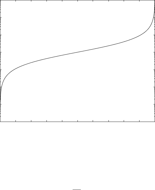
Figure 7.2 shows the exponential growth of the average queue size as the distri-

bution index increases. A semilog plot was chosen here to show in more detail the

size of the queue.

We can invoke Little’s result to estimate the wait time, which is the average num-

ber of time steps a packet spends in the queue before it is routed, as

= W ×Th (7.27)

where W is the average number of time steps that a packet spends in the queue.

Thus, W is given by

W =

a(1 −ρ)

(7.28)

232 7 Queuing Analysis

0 0.1 0.2 0.3 0.4 0.5 0.6 0.7 0.8 0.9 1

–4

–3

–2

–1

Distribution index (ρ)

Average buffer size

Fig. 7.2 Average queue size versus the distribution index ρ for the M/M/1 queue

This wait time is measured in units of time steps. The wait time in units of sec-

onds is given by the unnormalized version of Little’s result:



(7.29)

Example 7.1 Consider the M/M/1 queue with the following parameters a = 0.6

and c = 0.8. Find the equilibrium distribution vector and the queue performance.

From (7.7), the transition matrix is

P =

⎡

⎢

⎣

0.88 0.32000···

0.12 0.56 0.32 0 0 ···

00.12 0.56 0.32 0 ···

000.12 0.56 0.32 ···

0000.12 0.56 ···

00000.12 ···

⎤

⎥

⎦

The steady-state distribution vector is found using (7.17):

s =



0.625 0 0.234 4 0.087 9 0.033 0 0.

012 4 0.004 6 0.001 7 ···



7.6 M/M/1/B Queue 233

The probability of being in state i decreases exponentially as i increases.

The queue performance is as follows:

Th = 0.6 packets/time step

η = 1

= 0.6 packets

W = 1 time steps

Example 7.2 Investigate the queue in the previous example when the arrival proba-

bility is very close to the departure probability.

For the queue to remain stable, we must have a < c. Let us try a = 0.6 and

c = a + 0.01. The steady-state distribution vector is found using (7.17):

s =



0.0410 0.0393 0.0377 0.0361 0.0347 0.0332 0.0319 ···



Comparing this distribution vector with its counterpart in the previous example,

we see that the probability of being in state i is increased for i > 0. This is an

indication that the queue is getting close to being unstable.

The queue performance is as follows:

Th = 0.6 packets/time step

η = 1

= 23.4 packets

W = 39 time steps

We see that the throughput is increased since the probability that the queue is

empty (state 0) is decreased.

7.6 M/M/1/B Queue

This queue is similar to the discrete-time M/M/1 queue except that the queue has

finite size B. The state transition diagram is shown in Fig. 7.3.

Since packet arrivals and departures are independent of the time index value, we

have a homogeneous Markov chain. We assume that when a packet arrives, it could

Fig. 7.3 State transition

diagram for the discrete-time

M/M/1/B queue

0 1 2

adad1-ad

...

1-bcadad

bcbc

B-1

234 7 Queuing Analysis

be serviced at the same time step and it could leave the queue with probability c.

This results in the transition matrix given by

P =

⎡

⎢

⎣

bc 0 ··· 00 0

ad f bc ··· 00 0

0 ad f ··· 00 0

000··· fbc 0

000··· ad f bc

000··· 0 ad 1 −bc

⎤

⎥

⎦

(7.30)

where f

= 1 −ad and f = ac +bd.

Since the dimension of P is arbitrary, we are going to obtain an expression for

the equilibrium distribution vector s using difference equations techniques. The dif-

ference equations for the state probability vector are given by

ad s

−bc s

= 0 (7.31)

ad s

− gs

+bc s

= 0 (7.32)

ad s

i−1

− gs

+bc s

i+1

= 00< i < B (7.33)

where g = ad +bc and s

is the component of the distribution vector corresponding

to state i.

The solution to the above equations is given as













and in general,





i ≥ 0

It is more convenient to write s

in the form

= ρ

0 ≤ i ≤ B (7.34)

where ρ is the distribution index for the M/M/1/B queue:

ρ =

7.6 M/M/1/B Queue 235

The complete solution is obtained from the above equations plus the condition



i=0

= 1, which gives



i=0

= 1 (7.35)

from which we obtain s

, which is the probability that the queue is empty,

1 −ρ

B+1

(7.36)

and the equilibrium distribution for the other states is given from (7.34) by

(1 −ρ)ρ

1 −ρ

B+1

0 ≤ i ≤ B (7.37)

Note that ρ for the finite-sized queue can be more than one. In that case, the

queue will not be stable in the following sense:

< s

···< s

(7.38)

This indicates that the probability that the queue is full (s

) is bigger than the

probability that it is empty (s

7.6.1 M/M/1/B Queue Performance

The throughput or output traffic for the M/M/1/B queue is given by

Th = N

(out)

= ac s



i=1

= ac s

(

1 −s

)

= c

(

1 −bs

)

(7.39)

This throughput is measured in units of packets/time step. The throughput in

units of packets/s is



(7.40)

The input traffic is given by

(in) = 1 ×a +0 ×b = a (7.41)

236 7 Queuing Analysis

Input traffic is measured in units of packets/time step.

The efficiency of the M/M/1/B queue is given by

η =

(out)

(in)

(

1 −bs

)

(7.42)

Data are lost in the M/M/1/B queue when it is full and packets arrive but does

not leave. The average lost traffic N

(lost) is given by

(lost) = s

ad (7.43)

The above equation is simply the probability that a packet is lost which equals

the probability that the queue is full, and a packet arrives, and no packets can leave.

Lost traffic is measured in units of packets/time step. The average lost traffic per

second is given by



(lost) =

(lost)

(7.44)

The packet loss probability L is the ratio of lost traffic relative to the input traffic

L =

(lost)

(in)

= s

d (7.45)

The average queue size is given by the equation



i=0

(7.46)

Queue size is measured in units of packets. Using (7.37), the average queue size

is given by

ρ ×



1 −(B + 1)ρ

+ Bρ

B+1



(

1 −ρ

)



1 −ρ

B+1



(7.47)

Figure 7.4 shows the exponential growth of the average queue size as the distri-

bution index increases (B = 10 in that case). The solid line is for the M/M/1/B

queue and the dotted line is for the M/M/1 queue for comparison. We see that Q

for the finite-sized queue grows at a slower rate with increasing distribution index

compared to the infinite-sized queue. Furthermore, ρ for the infinite-sized queue

could increase beyond unity value.

7.6 M/M/1/B Queue 237

0.5 1 1.5 2 2.5 3

Distribution index (ρ)

Average buffer size

Fig. 7.4 Average queue size versus the distribution index ρ for the M/M/1/B queue when B = 10

(solid line). The dotted line is average queue size for an infinite-sized M/M/1 queue

We can invoke Little’s result to estimate the average number of time steps a

packet spends in the queue before it is routed as

= W ×Th (7.48)

where W is the wait time, or average number of time steps, that a packet spends in

the queue. The throughput in the above expression for the wait time must be in units

of packets time step. The wait time is simply

W =

(7.49)

Wait time is measured in units of time steps. The wait time in units of seconds is

given by



seconds (7.50)

Example 7.3 Consider the M/M/1/B queue with the following parameters a =

0.6, c = 0.8 and B = 4. Find the equilibrium distribution vector and the queue

performance.