Flechtner F.M., Gruber Th., G?ntner A., Mandea M., Rothacher M., Sch?ne T., Wickert J. (Eds.) System Earth via Geodetic-Geophysical Space Techniques
Подождите немного. Документ загружается.


504 M. Mandea et al.
radial direction and (θ,φ,r,t) is given by:
(θ, φ,t) = r
L
l,m
α
m
l
(t)Y
m
l
(θ, φ) (23)
These equations, corresponding to the radial FAC, lead to a purely tangential
field that contains all SH degrees up to L and therefore it cannot be separated from
the internal field unless the three components of the vector data are used. The SH in
Eq. (23) can be replace by a series of localized function F
i
(θ, φ) (see for example
Lesur, 2006) defined by:
F
i
(θ, φ) =
L
l,m
f
1
Y
m
l
(θ
i
,φ
i
)Y
m
l
(θ, φ) (24)
where the f
l
are chosen such that the gradients of the function F
i
(θ, φ) vanish rapidly
away from its centre (θ
i
,φ
i
). If f
l
for all l and if there is enough of these functions
then the expression 23 is equivalent to (see Lesur, 2006 for “exact equivalence”
rules):
(θ, φ,t) = r
i
α
i
(t)F
i
(θ, φ) (25)
Similarly, a model of the field generated in the ionosphere may be required and,
assuming the ionospheric currents are all flowing on a thin shell of radius, they are
defined by: J
io
= –η ×∇
s
(θ,φ,t) where the current function (θ ,φ,t) is given by:
(θ, φ,t) = r
io
L
l,m
β
m
l
(t)Y
m
l
(θ, φ) (26)
This flow of current give rise to a poloidal magnetic field that is therefore the
negative gradient of a potential V
io
(θ,φ,r). It is easy to establish that this potential is
related to the current function coefficients via:
V
io
(θ, φ,r,t) =
⎧
⎨
⎩
μ
0
r
io
l,m
l
2 l+1
r
io
r
l+1
β
m
l
(t)Y
m
l
(θ, φ)forr ≥ r
io
−μ
0
r
io
l,m
l+1
2 l+1
r
r
io
l
β
m
l
(t)Y
m
l
(θ, φ)forr ≤ r
io
(27)
where μ
0
= 4π10
–7
is the vacuum permeability. As above, this potential can be
written in terms of localised functions:
˜
F
i
(θ, φ,r,t) =
⎧
⎨
⎩
r
io
l,m
l
2 l+1
r
io
r
l+1
f
l
Y
m
l
(θ
i
,φ
i
)Y
m
l
(θ, φ)forr ≥ r
io
−r
io
l,m
l+1
2 l+1
r
r
io
l
f
l
Y
m
l
(θ
i
,φ
i
)Y
m
l
(θ, φ)forr ≤ r
io
(28)
and it is obtained:
V
io
(θ, φ,r,t) = μ
0
i
β
i
(t)
˜
F
i
(θ, φ,r) (29)
The Earth’s Magnetic Field 505
Separating the ionosphere contribution to the magnetic field from the field gen-
erated in the lithosphere and in the core is not easily done: the full vector data is
needed and also a sampling of the field at all local time.
Using CHAMP and observatory data (selected as indicated before), one of the
very high quality model available today is built, i.e. the GRIMM model (Lesur et al.,
2008). Using this model, a detailed picture of the core field and its secular variation
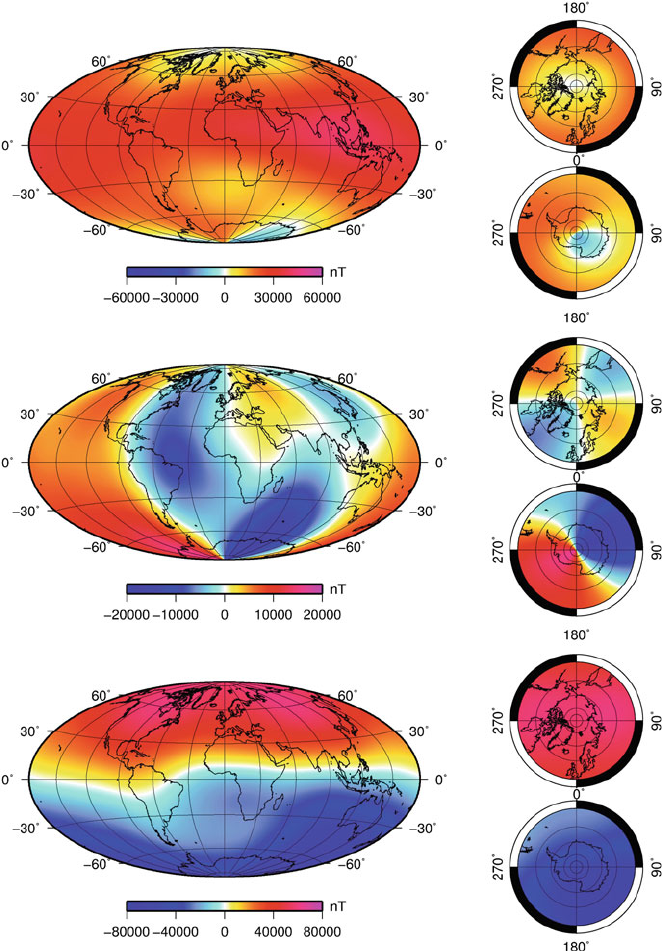
is obtained at the Earth’s surface. Figure 17 shows the global distribution of the
North, East and vertical downward components (X, Y, Z) of the geomagnetic core
field for the epoch 2003.25.
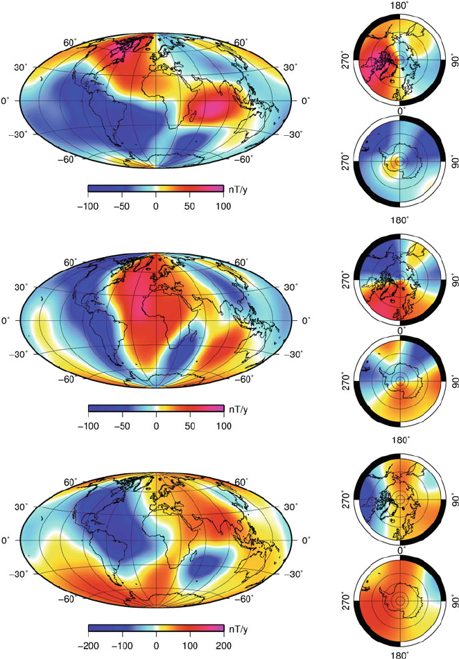
One of the remarkable achievements of the GRIMM model is its representation
of the temporal changes of the core field, i.e. its secular variation and acceleration.
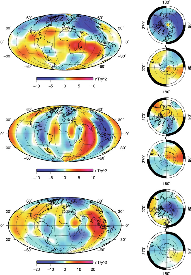
Figures 18 and 19 show these two quantities. Interestingly, the analyze of the sec-
ular acceleration indicates how rapidly the core field changes. This has enormous
implications for the core dynamics, that we do not discuss here, but the interested
reader is referred to Olsen and Mandea (2008) and Lesur et al. (2010).
Using the internal coefficients from a spherical harmonic analysis, is it possi-
ble to define the power spectra of the internal field (Lowes-Mauersberger spectra),
following (Lowes, 1966):
W(n) = (n + 1)
N
max
i
n=1
(g
m
n
)
2
+ (h
m
n
)
2
(30)
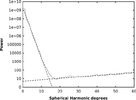
For example, using the MAGSAT vector data, it was clearly shown, for the first
time, that there is a major break in the power spectrum near spherical harmonic
degree 13 (Langel and Estes, 1985). This break is interpreted to represent the change
from dynamic core processes to quasi-static lithospheric ones. In Fig. 20 the power
spectrum obtained from a recent field model, GRIMM is shown. The steep part of
the spectrum (n ≤ 13) is clear and indicates the signature of the long wavelengths of
the core field, the transition degrees (n = 13–15) can be attributed to signals from
both the core and the crustal sources, and the higher degrees (n ≥16) are dominantly
lithospheric in origin.
3.3 Regional Modeling
For describing of the magnetic field at regional scales, methods such as the Spherical
Cap Harmonic Analysis have been proposed (Haines, 1985) and the related trans-
lated origin spherical cap harmonic analysis (De Santis, 1991), have been developed
to model the field over small patches of the globe. Korte and Constable (2003) have
pointed out that, the basis functions are not orthogonal, so it is not possible simul-
taneously to represent the potential for the vertical and horizontal field components,
exactly. Thébault et al. (2004) and Thébault et al. (2006b) have re-posed SCHA
as a boundary value problem within a cone extending above the reference surface,
thereby allowing satellite data to be downward continued to the Earth’s surface.
506 M. Mandea et al.
Fig. 17 Maps of the geomagnetic core field components, at the Earth’s surface: north compo-
nent (top), east component (middle), vertical downward component (bottom). Moldwide and polar
projections
The Earth’s Magnetic Field 507
Fig. 18 Maps of the secular variation components, at the Earth’s surface: north component (top),
east component (middle), vertical downward component (bottom). Moldwide and polar projections
508 M. Mandea et al.
Fig. 19 Maps of the secular acceleration components, at the Earth’s surface: north component
(top), east component (middle), vertical downward component (bottom). Moldwide and polar
projections
The Earth’s Magnetic Field 509
Fig. 20 The power spectrum obtained from the GRIMM model: the steep part of the spectrum
(n ≤ 13) indicates the core field contribution, the transition degrees (n =13–15) can be attributed to
both core and lithospheric contributions, and the higher degrees (n ≥ 16) describe the lithospheric
contribution. Units are in nT
2
This representation has been successfully applied for regions as small as the French
Metropolitan territory (Thébault et al., 2006a).
Basis functions, such as harmonic splines (Shure et al., 1982), or with more local
support, wavelet-like functions (Lesur, 2006) are better suited to data sets with vari-
able resolution over the globe. Recently, lots of efforts have been made in developing
new tools to describe the geomagnetic field at regional scale. They are based on
the wavelet frames and the pioneering work by Holschneider et al. (2003). In the
following the main aspects of this approach are described.
3.3.1 Wavelet Frames
The wavelets frames have been used to model the Earth’s magnetic field, as the
frame concept is more general than the basis one. The elements of a frame do
not need to be linearly independent, therefore the representation into a frame is
no longer unique.
The potential V of the magnetic field is expressed by the following superposition
of Poisson wavelets g
i
:
V(x) =
W
i=1
α
i
g
i
(x), (31)
where W is the finite number of wavelet, α
i
are unknown coefficients and x is the
evaluation point.

510 M. Mandea et al.
A Poisson wavelet on the sphere (Holschneider et al., 2003) is defined as:
g
(d)
y
(x) =
1
x
∞
l=0
|y|
|x|
d
Q
l
x.y
|x||y|
, (32)
where y is the position of the mathematical source, d is the scale of the wavelet
and Q
l
= (2 l + 1)P
l
is the reproducing kernel on the sphere, with P
denot-
ing the Legendre polynomials. A discretization of the mathematical sources of the
wavelets is applied (Holschneider et al., 2003; Chambodut et al., 2005) to obtain a
set of wavelets, which suitably covers the space and frequency domains. The sum
is infinite because the developing is around the centre of the Earth. If instead, a
development around the point x is used, the infinite sum becomes finite and:
g
d
y
(x) =
d+1
l=0
(2α
d+1
l
+ α
d
l
)
Rl!|x|
l
P
l
(
x−y·ˆy)
|x−y|
l+1
= ( −1)
d+1
d+1
l=0
(2β
d+1
l
− β
d
l
)
Rl!|y|
l
P
l
(
y−x·ˆx)
|x−y|
l+1
.
(33)
The coefficients α and β have a simple recursive expression, which may be
implemented efficiently, as the coefficients α
l
d
are recursively defined through:
α
d
l
= α
d−1
l−1
+ lα
d−1
l
, d ≥ 1
α
0
k
= δ
k,0
.
(34)
The coefficients β
l
d
are recursively defined through
β
d
l
= β
d−1
l−1
+ (l + 1)β
d−1
l
, d ≥ 1
β
0
k
= δ
k,0
.
(35)
3.3.2 Inverse Problem
Let us consider
b
i
, the values of the magnetic field at some observation points
x
i
, with i=1,...,M (typically at the satellite level). Usually, these values are con-
taminated with some errors. It is meaningful to suppose known
i,j
, the 2-point
correlation matrix of the errors, and (b) – a quadratic form providing some a
priori information about the magnetic field (for example, the quadratic form may
incorporate the average decrease of spectral energy of the field).
The problem which has to be solved is to find a minimizer α of the following
expression:
(Aα −b)
T
−1
(Aα −b) + λ(b), (36)
The Earth’s Magnetic Field 511
where A is the matrix containing the values of the wavelets at measurement
points, α is the unknown vector of the wavelet coefficients and λ is a Lagrange
multiplier.
3.3.3 Local Multipole Approximations
In order to take advantage of the properties of the Poisson wavelets (their local-
ization in space and frequency and their smoothness at the satellite altitude), each
wavelet can be approximated, within a given unity-volume P
j
, by its local multipole
expansion around the centre of mass x
0,j
of the M
j
data points inside it.
For a fixed unity-volume P
j
, a Poisson wavelet is approximated by:
g
d
y
(x) ≈
L
=0
m=−
c
m
h
Y
m
(β,γ ), (37)
where L is the degree of the multipole development, c
m
are constant coefficients,
Y
m
l
are again the spherical harmonics of degree l and order m, and (h,β,γ)arethe
spherical coordinates of the point
x −x
0,j
.
Using the approximation (37) the original inverse problem (36) gets the follow-
ing form:
(
˜
A ˜α − b)
T
−1
(
˜
A ˜α − b) +λ(b). (38)
In the above formulation, the matrix à can be represented as:
˜
A = C, (39)
where is a (M ×K[(L +1)
2
]) block-diagonal matrix, containing the values of the
local functions from (37) and C is a (K[(L + 1)
2
] × W) full matrix containing the
local coefficients.
Considering this decomposition of the matrix Ã, the problem (38) can be re-
written in the following form:
(C ˜α − η)
T
S(C ˜α − η) + λ(b),
where
S =
T
−1
η = S
−1
T
−1
b.
(40)
The simplest possible case is when L = 0. It is equivalent of approximating the
Poisson wavelets by piecewise constant functions and replacing the data by their
averaged values over each unity-volume.
This suggests that it is possible to considerably reduce the size of the original
problem involving the big system matrix A, with a new one which has a smaller sys-
tem matrix C. Obviously, a trend should be found between the gain of time and the
computational power of the inverse problem and the accuracy of the representation
of the data.
512 M. Mandea et al.
The first numerical tests, performed on CHAMP satellite magnetic data, allowed
us to check the behavior of the icosahedral volume implementation and furthermore
the applicability of the mathematical method.
In the two previous sections, the accent has been put on the magnetic data and
tools to model them. The given details are crucial for describing the part of the geo-
magnetic field originating in the lithosphere. This field, at global and some regional
scales is discussed in the following section. This is indeed one of the main topic of
this contribution.
4 Lithospheric Field: More Details at All Scales
The lithospheric contribution of the geomagnetic field has to be modeled by com-
bining satellite with ground-based, airborne and marine magnetic data in order to
describe all resolvable wavelengths. A prior thorough analysis of the available data
is necessary to detect outliers, incorrect coordinate systems or shifts in the data
before merging them. Careful examination of the data suggests that near surface
compilations contain long wavelengths (> 400 km) that differ significantly, both in
strength and shape, from global lithospheric field models based on satellite data. In
contrast, the wavelengths smaller than 400 km are naturally attenuated at the satellite
altitude and the derived models of the lithospheric field are then not very accurate.
The satellite models are therefore used t o describe the large scale lithospheric con-
tribution on global scale. Thus, in the following the global and regional features of
the lithospheric field are separately addressed.
4.1 Lithospheric Field and Its Large Scale
The satellite missions brought significant improvements in retrieving the large-scale
magnetic signatures of the Earth’s crust and upper mantle. Due to the flight alti-
tude of satellites it is impossible to resolve small-scale field structures from satellite
data. Indeed, a limitation inherent to magnetic surveys from satellites is that the
measurements have to be performed at a certain altitude. This implies that magnetic
features smaller than the orbit height cannot be resolved well because the spatial
decay of magnetic fields with distance from the source depends on spatial wave-
length. Considering recent satellites, with a typical altitude in average about 800 km
for Ørsted, 700 km for SAC-C and 400 km for the CHAMP mission, it is possible to
compute the impact of the orbit altitude on different wavelength features. The atten-
uation factors are listed in Table 2 for the spherical harmonic degrees 20, 50 and 80,
relative to observations at the Earth’s surface. From this table it becomes clear how
important measurements from low orbits are for high-degree magnetic field models.
Present improvements in the lithospheric field models are therefore based entirely
on CHAMP observations.

The Earth’s Magnetic Field 513
Table 2 Attenuation factors for small-scale crustal features (expressed by the SH degree) at
different orbital altitudes relative to amplitudes at the Earth’s surface
Altitude deg20 deg50 deg80
Surface 1 1 1
300 km 0.36 9.1 × 10
–2
2.3 × 10
–2
400 km 0.26 4.2 × 10
–2
6.8 × 10
–3
700 km 0.10 4.4 × 10
–3
1.9 × 10
–4
800 km 0.07 2.1 × 10
–3
6.1 × 10
–5
Nevertheless, high-degree spherical harmonic models are important for a number
of different purposes, like interpretation and identification of geological provinces
and tectonic boundaries (Ravat and Purucker, 2003), or large wavelength level-
ing of aeromagnetic surveys and marine survey track lines, or also, reduction of
crustal magnetic field signatures in studies of other field contributions. As men-
tioned before, spherical harmonic around degrees 13–15 core and lithospheric field
contributions have similar amplitudes. Inverse models therefore typically start at
spherical harmonic degree 16, while forward models include estimates of the longer
wavelengths.
The first high-degree internal models, also called lithospheric field models, have
been obtained from POGO and MAGSAT data. Due to the short MAGSAT mis-
sion duration and limitations of the only scalar data provided by the POGO series,
reliable expansions only up to degrees between 45 and 60 could be achieved
(Cain et al., 1989; Arkani-Hamed et al., 1994; Ravat et al., 1995). Advances
came along with the low-orbit CHAMP mission. The first version of a fam-
ily of high-degree models (MF), based on only one year of CHAMP scalar
data, provided a magnetic anomaly map valid at an altitude of 438 km and for
spherical harmonic degrees 14–65 (Maus et al., 2002). Many prominent crustal
magnetic features could already be identified on this map (some of them being
discussed in the following). With the following versions the vector field data
were also considered, allowing for upward/downward continuations of the model.
Downward continuation, however, has to be regarded with caution, as any noise
in the data contributing to the model is strongly amplified by this process. The
corresponding amplification factors for different altitudes can be inferred from
Table 2.
The GRIMM model also has a lithospheric contribution. Figure 21 shows the
GRIMM (Lesur et al., 2008), xCHAOS (Olsen and Mandea, 2008) and MF5 (Maus
et al., 2007) power spectra for the spherical harmonic degrees 16–60. Even, if both
the GRIMM and xCHAOS models are focused on the core field, they nonetheless
present similar spectra up to SH degree 45. This is an improvement compared to the
correlation between CHAOS and the BGS/G/L/0706 model (Thomson and Lesur,
2007) and it clearly confirms that not only t he MF5 lacks power, but also presents
spurious features at these l ow degrees.