Flechtner F.M., Gruber Th., G?ntner A., Mandea M., Rothacher M., Sch?ne T., Wickert J. (Eds.) System Earth via Geodetic-Geophysical Space Techniques

Подождите немного. Документ загружается.

Part VII

MAGFIELD

The Earth’s Magnetic Field at the CHAMP

Satellite Epoch

Mioara Mandea, Matthias Holschneider, Vincent Lesur, and Hermann Lühr

1 Introduction

The story of geomagnetism begins centuries ago with the ﬁrst ideas suggesting that

the Earth’s magnetic ﬁeld, itself, resembles a giant magnet. Like a conventional

magnet, our Planet has two magnetic poles, which do not coincide with the geo-

graphic poles. At the magnetic poles, a compass needle stands vertically pointing

either directly towards or away from the magnetic centre of the Earth. A bar mag-

net loses its magnetic properties over time, but the Earth’s magnetic ﬁeld has been

around for billions of years, so something is sustaining it. In reality the Earth dif-

fers from a solid magnet, and its magnetic poles are in constant motion as a result

of continual ﬂuid convections in its outer core. A century ago, Einstein stressed

that the origin of the Earth’s magnetic ﬁeld was one of the greatest mysteries of

physics. While our comprehension of the Earth’s magnetic ﬁeld has remarkably

improved, the self-sustaining, and somehow chaotic, nature of the Earth’s magnetic

ﬁeld remains poorly understood.

At the Earth’s surface, a compass needle swings until it aligns along a magnetic

North-South direction. In reality, t he Earth’s magnetic ﬁeld has a more complex

geometry than a pure North–South axial dipole. Traditionally, and for obvious

reasons, magnetic observations have been made at the Earth’s surface. The mag-

netic ﬁeld is thus commonly described in a local reference frame, either using the

Cartesian (X – north, Y – east and Z – vertical downward) components, or the angles

D, I (declination and inclination).

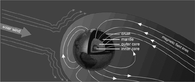
Nowadays, it is well-known that the observed Earth’s magnetic ﬁeld is the sum of

several internal and external contributions (Fig. 1). The dipole dominated core ﬁeld

is more than one order of magnitude stronger than the other contributions (Langel,

1987). This main part of the geomagnetic ﬁeld is believed to be generated by con-

vective motion in the Earth’s iron-rich, electrically conducting, ﬂuid outer core, by

M. Mandea (B)

Helmholtz Centre Potsdam, GFZ German Research Centre for Geosciences,

Department 2: Physics of the Earth, Telegrafenberg, 14473 Potsdam, Germany;

Now at Universitee Paris Diderot, Institut de Physique du Globe de Paris, France

e-mail: mioara@gfz-potsdam.de

475

F. Flechtner et al. (eds.), System Earth via Geodetic-Geophysical Space Techniques,

Advanced Technologies in Earth Sciences, DOI 10.1007/978-3-642-10228-8_42,



Springer-Verlag Berlin Heidelberg 2010

476 M. Mandea et al.

Fig. 1 Contributions in the Earth’s magnetic ﬁeld are internal (outer core and crust (lithosphere))

and external (ionosphere and magnetosphere) in origin

a process known as the geodynamo. This process is not fully understood, because a

few indirect observations exist to constrain it, only. According to the dynamo the-

ory, the observed magnetic ﬁeld is a product of this process, and its structure within

the core is very complex. This geodynamo generated ﬁeld is named core ﬁeld or

main ﬁeld, and its temporal variation, over time scales from decades to centuries,

is named secular variation. So, one can consider that the core ﬁeld morphology at

the Earth’s surface is relatively simple, being dominated by a dipole-like ﬁeld, incli-

nated with respect of the Earth’s rotation axis, and which accounts for some 90% of

the total ﬁeld.

The lithospheric (crustal) magnetic ﬁeld, with its origin in the remanent and

induced magnetization of the crust and upper mantle, is not only weaker, but also

of much smaller spatial scale, when compared to the large scale core ﬁeld. Its com-

plexity goes back to geological and tectonic origins (Mandea and Purucker, 2005),

and depends on magnetic minerals, mainly magnetite with varying content in tita-

nium. The titano-magnetite constituents have a Curie temperature in order of some

600

◦

C, above which they become essentially non-magnetic. Therefore, the litho-

spheric magnetization is limited to a layer of about 7–50 km in thickness, depending

on the local heat ﬂow.

The Earth’s magnetic external ﬁelds stem from the interaction with the solar

wind, which compresses the magnetic ﬁeld lines on the sunward side and stretches

them into a long tail on the night side. Generally, solar wind particles do not cross

ﬁeld lines and are thus primarily deﬂected around our planet. They may, however,

enter the magnetosphere when interplanetary and geomagnetic ﬁelds merge during

times of increased solar activity, or close to poles where t he ﬁeld-lines are nearly ver-

tical. Their interaction with the atmosphere then causes the well-known aurora. For

more information on the geomagnetic ﬁeld contributions and variations the reader

is referred to Gubbins and Herrero-Bervera (2007) and Glassmeier et al. (2009).

An important feature of the geomagnetic ﬁeld is its variability on many different

time scales, from less than a second to millions of years (Mandea and Purucker,

2005). It even changes its polarity. This knowledge relies on various data sources,

The Earth’s Magnetic Field 477

ranging from rock magnetization measurements to historic magnetic measurements,

and even recent high-quality data provided by magnetic observatories and the mag-

netic satellites MAGSAT, Ørsted, CHAMP and SAC-C, (Lühr et al., 2009). The

combination of ground and continuous satellite measurements allows the core mag-

netic ﬁeld and its time variation to be described with a very high resolution in space

and in time (Lesur et al., 2008; Olsen and Mandea, 2008). Recent dynamo simu-

lations have contributed signiﬁcantly to understand the core ﬁeld geometry and its

dynamics, and temporal changes, including excursions and reversals (Christensen

and Wicht, 2007; Wicht et al., 2008).

Since the magnetic ﬁeld changes in space and time, magnetic observations must

continually be made, on ground and in space, and models are generated to accurately

represent the magnetic ﬁeld as it is. One of the most difﬁcult tasks is to separate

the internal contributions between the part produced in the core and the one pro-

duced by the lithosphere (Langel and Hinze, 1998). It is generally agreed that the

core contributions are well described up to degree and order 13, when spherical

harmonic analysis is used as modeling tool. However, as it has been pointed out

many times, features of the lithospheric magnetic ﬁeld with wavelengths in excess

of 3,000 km (spherical harmonic degree 13) are completely obscured by the overlap-

ping core ﬁeld. Between 2,600 and 3,000 km both core and lithospheric signatures

are present, hindering efforts for their separation (Mandea and Thébault, 2007). No

method has been found yet to separate completely the two sources. The general

practice has been to ignore the crustal contribution below degree 13, and core com-

ponent above degree 16 (see below). Generally speaking, the previous efforts at

their separation of the two ﬁelds have failed, and there is a strong reason to believe

that the two ﬁelds are not completely separable, unless the core ﬁeld is shut off or

changed signiﬁcantly.

However, recently large improvements have been achieved in resolving the

Earth’s lithospheric ﬁeld with spatial scales reaching down to a few hundreds of

km in the satellite component of the recently published World Digital Magnetic

Anomaly Map (Korhonen et al., 2007). In the following we focus on this ﬁeld

component, with more details on used data (from ground and space platforms), the

mathematical tools to represent them (on global and regional scales), and ﬁnally the

new lithospheric ﬁeld models and their contributions to a better understanding of

the tectonic and geological features.

2 Ground and Space Measurements

Two types of measurements are needed to characterize the geomagnetic ﬁeld: scalar

and vector. The Overhauser magnetometer, a type of proton precession or resonance

magnetometer, is typically installed at magnetic observatories, but is also used for

some other ground observations and on the Ørsted and CHAMP magnetic satellites.

In contrast, vector measurements made with a ﬂuxgate magnetometer are subject

to instrument drift. To minimize this drift contribution in the ﬁnal data, different

approaches are used for ground or satellite measurements.

478 M. Mandea et al.

2.1 Ground Measurements

2.1.1 Magnetic Observatories

Historically, magnetic observatories were established to monitor the secular change

of the Earth’s magnetic ﬁeld, and this remains one of their most important functions.

This generally involves absolute measurements that are sufﬁcient in number to mon-

itor instrumental drift of ﬂuxgate magnetometers giving variation measurements

of the three ﬁeld components. Over 70 countries operate some 200 observatories

worldwide.

A scalar measurement of the ﬁeld intensity obtained commonly by a proton mag-

netometer is absolute: this means it depends only on our knowledge of a physical

constant and a measurement of frequency, and can be achieved with great accuracy

(in excess of 10 ppm). Scalar magnetometers make measurements of the strength

of the magnetic ﬁeld only, and provide no information about its direction. It is also

possible to make an absolute measurement of the direction of the geomagnetic ﬁeld

with respect to the horizontal plane (I – inclination) and the angle in the horizontal

plane between the magnetic North and true North (D – declination). This can only be

performed with an instrument known as a ﬂuxgate-theodolite (DI-ﬂux) that requires

manual operation and takes about 15 min per measurement. The DI-ﬂux consists

of a non-magnetic theodolite and a single-axis ﬂuxgate sensor mounted on top of a

telescope. The DI-ﬂux is considered to be an absolute instrument, which means that

the angles measured by the instrument do not deviate from the true values D and I.

This is achieved by using an observation procedure that eliminates unknown param-

eters such as sensor offset, collimation angles and theodolite errors. In a land-based

observatory, such absolute measurements are typically made once/twice a week and

are used to monitor the drift of the ﬂuxgate variometers.

A vector measurement made with a ﬂuxgate magnetometer is subject to instru-

ment drift arising from sources both within the instrument (e.g. temperature effects)

and also the stability of the instrument mounting. Because these measurements are

not absolute, they are referred to as variation measurements, and the instruments are

known as variometers. One of the most widely used variometers is the FGE ﬂux-

gate manufactured by the Danish Meteorological Institute, Denmark. The sensor

unit consists of three orthogonally mounted sensors on a marble cube. In order to

improve long-term stability, these sensors have compensation coils wound on quartz

tubes, resulting in a sensor drift of only a few nT per year. The marble cube is sus-

pended by two strips of crossed phosphor-bronze working as a Cardans suspension

to compensate for pillar tilting that might cause baseline drift. The box containing

the electronics is almost magnetic free, and is placed several meters from the sensor

to further minimize its effect on the readings. Measurements are made by apply-

ing an alternating magnetic ﬁeld to a material of high-magnetic permeability. The

voltage induced in a pickup coil is then measured, and the resulting even harmonics

are proportional to the ambient magnetic ﬁeld in the direction of the coil winding.

The magnitude and directional response of these instruments needs to be calibrated

against accurately known sources.

The Earth’s Magnetic Field 479

All modern land-based magnetic observatories use similar instrumentation to

produce similar data products. For a full description, see Jankowski and Sucksdorff

(1996) and also the INTERMAGNET web site.

The fundamental measurements

recorded are averaged 1-minute values of the vector components and of scalar

intensity. The 1-minute data are important for studying variations in the geomag-

netic ﬁeld external to the Earth, in particular the daily variation and magnetic

storms. Data from a sub-network of observatories are used to produce the Kp

and magnetic activity indices. From the 1-minute data, hourly, daily, monthly and

annual mean values are produced. The monthly and annual mean values are used to

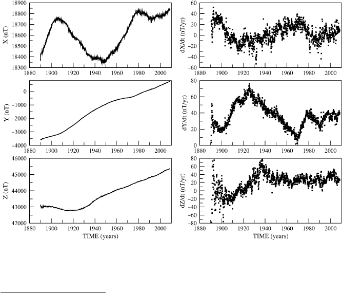
determine the secular variation emulating from the Earth’s core. Figure 2 shows

the magnetic ﬁeld evolution for the three components (X, Y, Z), and the corre-

sponding secular variation, measured at Niemegk observatory (Germany). It is

very clear that the quality of secular-variation estimates (sometimes of the order

of a few nT/yr) depends critically upon the quality of the measurements at each

observatory.

Installed mainly on continents, the magnetic observatories are very unevenly and

sparsely distributed. This is the reason why in some regions, as for example the

Paciﬁc, the ground-data based models uncertainty is very large. One possibility for

Fig. 2 Temporal evolution of the monthly means for the X, Y, Z components and the correspond-

ing secular variation, recorded at Niemegk observatory (Germany)

www.intermagnet.org

480 M. Mandea et al.

improving the geomagnetic models in such areas is to consider some other sources

of data, as those provided by repeat stations or by satellites.

2.1.2 More Ground or Near-Earth Measurements

The network of repeat stations. Because of the temporal changes in magnetic ﬁeld

and the uneven distribution of observatories, at national level repeat station net-

works exists. However, this is not true everywhere: for example there is not such

a network in Russia or in all Central African regions. For a repeat station survey

three components of the geomagnetic ﬁeld are measured (generally the two angular

components and the total intensity) at several well-deﬁned points distributed across

the considered region. However, unlike at geomagnetic observatories, the ﬁeld is

not continuously recorded, measurements are made at best once per year, often only

every 5 years. To obtain ﬁnal data that is comparable to those provided by the geo-

magnetic observatories, speciﬁc data reduction methods have to be applied. Repeat

station data offer better spatial resolution than do observatory data alone, and they

are used for a better spatial resolution in global magnetic modeling, lithospheric

induction, and conductivity studies, reduction of aeromagnetic surveys, and for

describing the lithospheric ﬁeld (although much denser station networks are needed

for that task).

Aeromagnetic surveys. For studying the lithospheric ﬁeld, detailed features of the

magnetic ﬁeld are required. They are so complicated that observatory or repeat sta-

tion measurements alone are not adequate. Moreover, dense ground measurements,

when existing, are generally inappropriate because of the irregular surface topogra-

phy and the surface anthropogenic activity that creates artiﬁcial magnetic sources in

many different places. Therefore, measurements at ﬁxed aircraft altitude and along

regular proﬁles are more convenient. It is extremely difﬁcult to point a ﬁxed direc-

tion is space, and therefore, aeromagnetic surveys usually record the strength of the

magnetic ﬁeld; i.e. they are scalar measurements. Aeromagnetic surveys are fast,

which reduces the secular variation problem for a given survey. The external ﬁeld

variations are reduced using the nearest magnetic observatory or a ﬁxed base station

set up especially for the survey. Aeromagnetic surveys are usually a few kilome-

ters to hundreds kilometers. They are carried out for a variety of purposes. Fields

of research include, for instance, investigation of crystalline basement and mineral

exploration, for fault and fracture zones or for imaging volcanic structure. Large

aeromagnetic surveys with wider proﬁle spacing are devoted to both regional and

detailed geological investigations over landmass and continental shelves. They can

provide information about the distribution of rocks occurring under thin layers of

sedimentary rocks, useful when trying to understand geological and tectonic struc-

tures. However, the aeromagnetic measurements are not useful in constraining the

secular variation of the core ﬁeld. As this kind of data is largely used in obtaining a

global view of the lithospheric ﬁeld, more details about the aeromagnetic data, their

processing and use are given in the following.

The Earth’s Magnetic Field 481

2.2 Satellite Measurements

Since the 1960s, with the American OGO series of satellite, the Earth’s mag-

netic ﬁeld intensity has been measured intermittently from space at altitudes

varying from some 400–1,500 km. The main advantages of satellite compared

to airplane are its capability to measure the magnetic ﬁeld over a rather long

period, at a relatively constant altitude and to provide a homogeneous data distri-

bution. Moreover, data are obtained with the same instrument characteristics. In

the following, it is illustrated that these properties are extremely valuable for the

magnetic ﬁeld modeling in general and, more precisely, for the lithospheric ﬁeld

description.

The ﬁrst satellite mission that provided vector data for geomagnetic ﬁeld mod-

eling was initiated by the National Aeronautics and Space Administration (NASA).

The MAGSAT satellite (Langel et al., 1980) operated over a 6-month period

between 1979 and 1980, a short period that provided the ﬁrst consistent, but low

resolution, map of the lithospheric ﬁeld. The following 20 years lacked of high-

quality magnetic ﬁeld missions, but the Danish Ørsted satellite,

launched in 1999,

improved the situation. However, the primary goals of the mission have been to

study the variations of the magnetic ﬁeld of the Earth and its interaction with the

sun particles stream. As a result, the satellite altitude is too high to provide us with

a high resolution view of the lithospheric ﬁeld sources.

Ørsted was followed by the German CHAMP (Challenging Minisatellite

Payload) satellite

and the SAC-C satellite with the Ørsted-2 experiment, launched

in July and November 2000, respectively. All three missions carry essentially the

same instrumentation and provide magnetic ﬁeld observations from space with

unprecedented accuracy. Due to the somewhat different altitudes (Ørsted: 630–

860 km, CHAMP: 310–450 km; SAC-C: ∼700 km) and drift rates through local

time, the spacecraft sense the various internal and external ﬁeld contributions

differently.

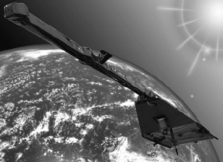
The most successful mission for magnetic ﬁeld studies is the CHAMP satellite

(Fig. 3), still fully operating in mid-2010, ten years after its launch. Its low-Earth

circular orbit is particularly suitable for crustal ﬁeld mapping. The initial average

satellite altitude was 454 km, but the satellite is slowly descending and reaches

330 km altitude in 2009. The lithospheric maps obtained from this satellite exper-

iment are the most robust and have an unprecedented resolution. In the following

example, when dealing with satellite data, we mainly rely on the CHAMP satellite

mission, and this satellite, its instruments, and data processing are discussed in more

detail.

http://www.spacecenter.dk/research/solarphysics/orsted

http://www.gfz-potsdam.de/portal/-?$part=sec23

482 M. Mandea et al.

Fig. 3 The CHAMP satellite

– photo of the real-size model

in Helmholtz-Zentrum

Potsdam Deutsches

GeoForschungsZentrum,

GFZ-Building H

2.3 CHAMP Data Processing

The CHAMP satellite carries a number of scientiﬁc instruments: the scalar

Overhauser Magnetometer (OVM), the vector Fluxgate Magnetometer (FGM) and

two dual-head star cameras (Advanced Stellar Compass, ASC), the Accelerometer

(ACC), the GPS receiver, the Digital I on Drift-Meter (DIDM). In addition, for pro-

cessing the readings of the scientiﬁc instruments, auxiliary information such as

temperatures, currents and the precise satellite orbit have to be derived from ded-

icated sensors. A data processing chain has been developed to routinely generate

Level 2 data from all the aforementioned instruments. A ﬁrst description of the pro-

cessing approach can be found in Rother et al. (2005). The CHAMP data are made

available through the Information System and Data Center (ISDC) at GFZ to the

community of approved co-investigators and registered data users.

Data are available at different processing levels, deﬁned in the “CHAMP

project”. Level 0 are raw data as received by the telemetry. These are densely packed

or even compressed in order to allow for an efﬁcient transmission. Level 1 products

are decoded and formatted but uncalibrated data, convenient to read by standard

codes. They contain the full information of measurements performed in space. Level

2 products are properly scaled and calibrated data, in physical units. Each of these

products can be related to a certain instrument. It has to be noted that the deﬁnition

of the processing levels in the “CHAMP project” is somewhat different from the

convention for ESA missions.

In the following some details of the processing steps which are applied for gen-

erating the magnetic ﬁeld Level 2 products are given. The description is ordered by

instruments, starting with the raw data, and presents the major steps to achieve the

Level 2 products.

2.3.1 Overhauser Magnetometer Data Processing

The CHAMP Overhauser magnetometer (OVM) is regarded as the magnetic

reference instrument. Its output frequency is directly proportional, through the

The Earth’s Magnetic Field 483

gyro-magnetic ratio, to the ambient magnetic ﬁeld magnitude. On this mission, it

samples the magnetic ﬁeld at a rate of 1 Hz with a resolution of 0.1 nT. In order

to make the readings a traceable standard, the output frequency is compared to a

reference oscillator.

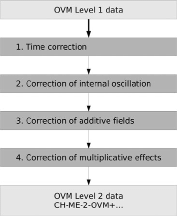
Although the OVM readings are highly accurate, they do not simply reﬂect the

Earth’s magnetic ﬁeld. There are magnetic inﬂuences from the spacecraft and the

instruments which have to be taken into account. The major processing steps for

correcting the data are outlined in Fig. 4.

The Level 1 data are the input for the processing. Each reading comes with a time

stamp, accounting for the time of transmission from the instrument to the on-board

data handling system (OBDH). For the data interpretation it is important to know

precisely the epoch at which the reading is valid. Since the satellite is a fast moving

platform (7.6 km/s), readings have to be time-tagged with millisecond precision.

The relevant time difference has been determined in ground tests. The epoch of the

OVM readings is deﬁned as the reference time to which the Level 2 data of all the

other instruments, relevant for the magnetic ﬁeld products, are resampled.

During the processing step 2 the applied scale factor to the magnetic ﬁeld read-

ings is checked and corrected. For determining the actual frequency of the internal

oscillator the cycles are counted within a gate of 60-GPS seconds. To convert the

Larmor frequency into magnetic ﬁeld strength, the gyro-magnetic ratio is applied,

as recommended by the International Association of Geomagnetism and Aeronomy

(IAGA), during the IUGG General Assembly in Vienna, 1991. With this convention

the CHAMP scalar magnetic ﬁeld readings can be traced back uniquely to the two

internationally maintained standards, GPS-second and gyro-magnetic ratio.

The remaining corrections concern the disturbances produced by the satellite. In

step 3, all ﬁelds adding to the true ambient are considered together. Contributions

Fig. 4 Schematic ﬂow chart

for the processing of the

overhauser magnetometer

data. For details of the

processing steps see the text