Flechtner F.M., Gruber Th., G?ntner A., Mandea M., Rothacher M., Sch?ne T., Wickert J. (Eds.) System Earth via Geodetic-Geophysical Space Techniques

Подождите немного. Документ загружается.

484 M. Mandea et al.

come from the remanent magnetization of the spacecraft, from electric currents in

the systems, and also from the directional anisotropy of the sensor. These extra ﬁelds

cannot be simply subtracted. Their inﬂuence on the ﬁeld magnitude has to be deter-

mined by ﬁnding the projection of the disturbance on the total ﬁeld vector. Only this

projection is considered in the correction. Since the external contributions are small

compared to the ambient ﬁeld, the corrections can be accomplished conveniently

using a scalar product between the disturbance vector b and the ambient magnetic

ﬁeld vector B

FGM

, measured by the FGM.

OVM

|=B

−

b ·B

FGM

,(1)

where |B

OVM

| is the total intensity ﬁeld corrected for disturbances and B

is the reading of the OVM. The disturbance vector b is the sum of several

contributions,

b = b

+ b

aniso

+ b

stray

+ b

torq

.(2)

The remanent magnetic ﬁeld of the spacecraft, b

, has been determined in a

pre-ﬂight system test. Since the OVM is mounted at the tip of a 4 m long boom, the

remaining effect is only of the order of 0.5 nT. Also the dependence of the OVM

reading on the direction of the ﬁeld vector, b

aniso

, is rather small (< 0.3 nT). There

are some stray ﬁelds, b

stray

, generated by electric currents, e.g. in the solar panels

which make effects of less than 0.5 nT. Current readings from the housekeeping data

are also needed for this correction. Comparably large are the contributions from

the three orthogonal magneto-torquers, b

torq

, which are used for controlling the

spacecraft attitude. These ﬁelds reach amplitudes of more than 3 nT at the position

of the OVM. Fortunately, they can be predicted quite reliably when the currents

through the torquer coils are measured.

torq

⎛

⎝

1,1

1,2

1,3

2,1

2,2

2,3

3,1

3,2

3,3

⎞

⎠

⎛

⎝

⎞

⎠

(3)

Where I

, I

are the currents through the three respective coils and q

n,m

are

the elements of the torquer correction matrix, which have to be determined in the

magnetic system test.

In step 4, corrections associated with perturbation proportional to the ambient

magnetic ﬁeld are considered. For CHAMP, these are the permeability of the space-

craft and the cross-talk from the FGM onto the OVM. For considering these effects,

a somewhat different approach is needed. Indeed,

OVM

|=B

− (dxB

+ dyB

+ dzB

)/B

(4)

where dx, dy, dz denote the modiﬁcations in the scaling factors in the vector

directions; B

, B

are again the ambient ﬁeld components as measured by the

The Earth’s Magnetic Field 485

FGM. The values of dx, dy and dz are for both effects, S/C permeability and FGM

cross-talk, of order 1 × 10

–5

. They have also been determined during the system

magnetic tests. Fortunately, all three components of the two contributions happen to

have similar amplitudes, but opposite signs. Therefore, the total disturbance caused

by multiplicative effects is largely cancelled.

After applying the described corrections to the OVM data, they are considered

Level 2 and transferred to the data center, ISDC. Based on the fairly small sizes of

the various correction terms described above one can conclude that the ﬁeld mag-

nitudes provided in this Level 2 product are rather reliable. Finally, it is considered

that an absolute accuracy of better than 0.5 nT is reached.

2.3.2 Fluxgate Magnetometer Data Processing

The ﬂuxgate magnetometer (FGM) measures the three components of the magnetic

ﬁeld. These vector ﬁeld measurements are performed at a rate of 50 Hz with a

resolution of 0.1 nT. This higher rate is justiﬁed by the signiﬁcantly larger variabil-

ity of vector components compared to the ﬂuctuations of the ﬁeld magnitude. The

FGM is an analogue instrument; therefore its characteristics are expected to change

in response to environmental inﬂuences or with time. In order to ensure reliable

readings of the vector ﬁeld components from a multi-year mission, the calibration

parameters have to be updated at regular intervals (for CHAMP this is done every

15 days). The in-ﬂight calibration is based on a direct comparison between of the

FGM readings with the OVM Level 2 data. Details of the calibration approach are

given below.

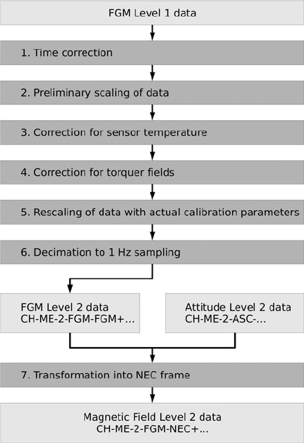
Figure 5 shows, in a similar way as Fig. 4, the main processing steps applied

to the FGM Level 1 data. It starts again with the proper dating of the readings

where the delay of the time stamp with regard to the exact epoch of measurement

is considered. In step 2 the raw data are converted to physical units with the help

of a preliminary set of parameters. The measurements are expected to have a bias

and need to be scaled. Firstly, the offset vector is subtracted from the FGM read-

ings, measured in engineering units. Thereafter, the results are scaled into nT. For

CHAMP, linear, quadratic and cubic terms are taken into account. As an example,

for the x component, one can write:

= S

− O

) +S

− O

)

+ S

− O

)

(5)

where B

is an estimation of the magnetic ﬁeld in the x direction, S

, S

are

the scaling factors, E

are the FGM readings in engineering units, and O

is the offset

in the x direction. The non-linear corrections have been determined in the laboratory

before the launch. They are rather small and thus considered to be constant over the

mission. Finally, the deviations of the sensor elements from the orthogonality are

corrected:

= C ·B

(6)

486 M. Mandea et al.

Fig. 5 Schematic ﬂow chart for the processing of the Fluxgate magnetometer data. For details of

the processing steps see the text

where C is the matrix correcting for the non-orthogonality. This matrix has the form

C =

⎛

⎝

1 cos (x,y) cox(x,z)

0 1 cos (y,z)

00 1

⎞

⎠

(7)

where the elements represent the cosine of the angle between respective sensor

elements.

Corrections of the environmental inﬂuences start with step 3. The sensor changes

its geometry with the ambient temperature. This has an inﬂuence on the scal-

ing factor. Other parameters, bias and sensor orientation, are not affected by the

temperature. In pre-ﬂight tests the temperature coefﬁcients have been determined.

The Earth’s Magnetic Field 487

They amount to about 30 ppm/K for all axes. This effect is corrected using the

temperature measurements at the sensor place.

During the step 4 the magnetic ﬁelds produced by the spacecraft are considered.

For the FGM, there is no need to correct for constant or slowly varying inﬂuences,

such as the remanent and induced magnetic ﬁeld of the spacecraft: these effects are

accounted for in the FGM calibration parameters. However, disturbances varying

over short time have to be corrected directly. An example of that is the magnetic

ﬁeld, B

torq

, caused by the t orquer coils.

torq

⎛

⎝

1,1

1,2

1,3

2,1

2,2

2,3

3,1

3,2

3,3

⎞

⎠

⎛

⎝

⎞

⎠

(8)

where p

n,m

are the elements of the torquer correction matrix for the FGM. As noted

before, these elements have been determined during the magnetic system tests. The

vector B

torq

has to be subtracted from the scaled FGM readings

FGM data corrected to this level are used for the scalar calibration. This cali-

bration against OVM data results in an improvement of the nine FGM processing

parameters (3 scale factors, 3 offset values, 3 angles between sensors). The fully

calibrated vector data, B

FGM

= B

+dB, are obtained in this way

dB =

⎛

⎝

cos (dx,y) cos (dx,z)

0 dS

cos (dy,z)

00 dS

⎞

⎠

.(B

− dO)(9)

where all the quantities preceded by a d are the corrections with respect of the

original values and B

as it has been deﬁned above.

So far, the processing scheme is applied to the full 50 Hz data set. Before con-

version to Level 2 products the vector data are re-sampled to 1 Hz, in order to make

them consistent with the scalar data (step 6). This re-sampling is not accomplished

by a simple average over the FGM reading within a second. A linear ﬁt to the 100

values centered on the target time has been preferred. The new value i s then com-

puted from the derived function at the epoch of the related OVM reading. This

procedure is performed individually for all three components.

The new data set is then a Level 2 product accessible through the ISDC. These

fully calibrated vector data are useful for certain applications, but they are given in

the FGM sensor frame. For that reason during s tep 7 a transformation of the data

into the commonly used NEC frame is done. NEC i s a local Cartesian frame having

its origin at the position of the satellite. The three components point to geographic

north, east and to the centre of the Earth, respectively. A number of rotations have

to be performed for this coordinate transformation:

NEC

= R

(NEC←ITRF)

· R

(ITRF←ICRF)

· R

(ICRF←ASC)

· R

(ASC←FGM)

· B

FGM

(10)

488 M. Mandea et al.

The rotation angles from the FGM sensor system to the star camera (ASC) are

determined before launch. The rotation into the celestial frame, ICRF, is based on

the Level 2 attitude data. For the rotation from the ICRF into the Earth-ﬁxed, ITRF

frame, the current Earth’s rotation parameters are used (as provided by the IERS ser-

vice), where the satellite position is taken from the precise orbit determination. The

ﬁnal rotation into the NEC frame requires just the satellite position. Magnetic ﬁeld

vector data in the NEC frame are the prime data source for all modeling efforts and

for various other applications. Therefore, this is the magnetic ﬁeld Level 2 product

most frequently downloaded from the ISDC.

2.3.3 In-Flight Scalar Calibration

When processing the FGM magnetic ﬁeld readings for a multi-year mission, in-

ﬂight calibration plays an important role. For that reason we present the approach

used for CHAMP and the results obtained over its ﬂight-time, in some more detail.

During the calibration process the readings of the OVM are used as a reference.

By comparing ﬁeld magnitude values with those from FGM, the nine principle

parameters of the vector instrument can be determined in a non-linear inversion.

The basic idea is that the OVM and FGM should provide the same values for the

magnetic ﬁeld strength, and any difference can be explained by an improvement of

the nine basic FGM parameters. These parameters are expected to be constant over

at least 1 day. In a linear approximation, it is required that

B = B

· dB = 2B

⎛

⎝

cos (dx,y) cos (dx,z)

0 dS

cos (dy,z)

00 dS

⎞

⎠

.(B

− dO) (11)

where B is the difference in the ﬁeld strength between OVM and FGM estimates.

Equation (11) represents a linear expression relating the processed OVM data to

the magnetic ﬁeld components f rom the FGM through the nine unknown. In prac-

tice, a system of equations is set up making use of all 86,400 daily measurements,

from which the nine FGM parameters are determined by least squares.

With a day of data, the FGM parameters are determined. Averages over 15 days

are used in the FGM processing for the ﬁnal scaling of the vector data. After this last

processing step the root mean square (rms) value of the difference between OVM

and FGM varies from 0.1 to 0.2 nT. This can be regarded as a veriﬁcation of the

used calibration approach.

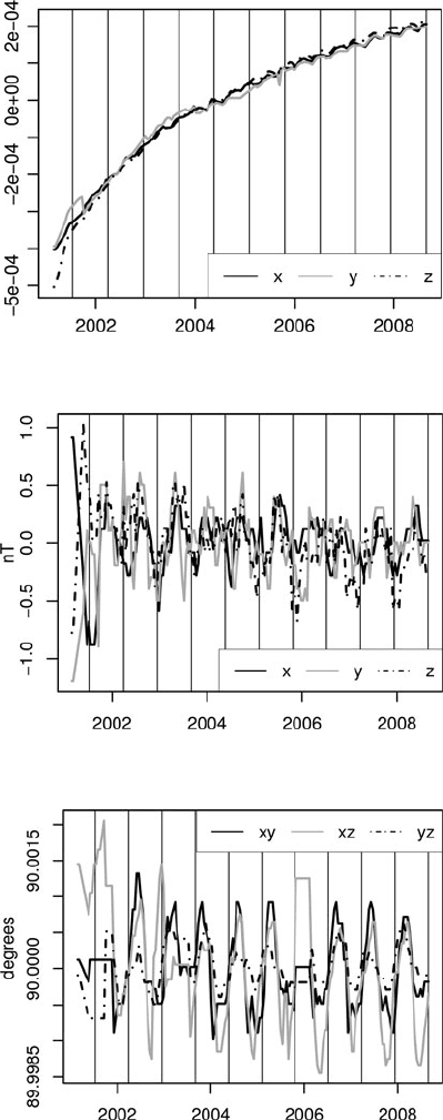
The CHAMP satellite has been in orbit for more than 8 years. It is thus inter-

esting to see how the prime FGM parameters have varied over the mission period.

In Figs. 6, 7, and 8 the long-term variations of the applied parameters are shown.

For the convenience of interpretation, vertical lines are drawn at times when the

ascending arc of the orbital plane coincides with the 6 o’clock local time sector,

and mean values are subtracted in order to allow a more direct comparison of the

The Earth’s Magnetic Field 489

Fig. 6 Temporal changes of

the Fluxgate magnetometer

scale factors. Mean values

have been subtracted. The

vertical lines indicate times

when the orbital plane is in

the 6 o’clock local time sector

Fig. 7 Temporal changes of

the Fluxgate magnetometer

offset values. The vertical

lines indicate times when the

orbital plane is in the 6

o’clock local time sector

Fig. 8 Temporal changes of

the angles between the

Fluxgate sensor axes. The

vertical lines indicate times

when the orbital plane is in

the 6 o’clock local time sector

490 M. Mandea et al.

Table 1 Mean values of the nine Fluxgate parameters, which have been substracted from the

curves plotted in the Figs. 6 and 7

plot

= b–b

offset

plot

offset

plot

bx 27.380

plot

by 20.695

plot

bz 21.374

anlge

plot

= angle – angle

offset

anlge

plot

angle angle

offset

plot

α 0.02588

plot

β 0.060247

plot

γ 0.038787

plot

= s–s

offset

plot

offset

plot

sx 1.002353

plot

sy 1.003278

plot

sz 1.003194

ﬁeld components. The values subtracted are listed in Table 1. There are system-

atic differences between the variations of the scale factors and the other parameters.

The scale values show a monotonic increase over time. The trend is the same for all

three components and it can reasonably well be approximated by a logarithmic func-

tion. Over the mission lifetime, the scale factor has changed by 7 parts in 10.000,

corresponding to an error in magnetic ﬁeld of some 40 nT.

The other parameters show no signiﬁcant long-term trend, but exhibit periodic

variations in phase with the orbit local time. Amplitudes of the offset variations

(Fig. 7) are generally smaller than 0.5 nT. Regarding the sensor stability (Fig. 8)

variations are conﬁned to angles of 0.001

◦

which correspond to 3.6 arcs. For these

six parameters the in-ﬂight calibration conﬁrms the high stability of the FGM instru-

ment on CHAMP. It should be noted here that the stability of the six parameters may

even be better than shown here. The synchronization of the deduced variations with

the orbital local time suggests that other, not corrected perturbations of the measure-

ments leak into these parameters. However, this does not affect the validity of the

Level 2 data.

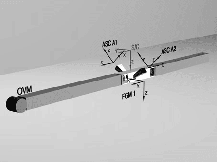
2.4 Advanced Stellar Compass Data Processing

For the scientiﬁc use of the vector measurements the orientation of the components

has to be known with high precision. To achieve t his goal CHAMP is equipped

with a special optical bench, which houses the FGM and two star camera head units

(CHU). The purpose of the optical bench is to provide a mechanically stable con-

nection between magnetometer and star tracker. Figure 9 shows schematically the

arrangement of the instruments on the boom and the orientation of the various coor-

dinate systems. The viewing direction of the two cameras is separated by 102

◦

The Earth’s Magnetic Field 491

Fig. 9 Schematic drawing of

the CHAMP boom and its

instrument assembly. Also the

orientations of the relevant

coordinate systems referred to

in the text are shown

Therefore, they survey two completely different regions of the sky, and the informa-

tion provided by the two camera heads are combined in order to improve the attitude

determination.

The Advanced Stellar Compass (ASC) is a sophisticated instrument, performing

self-consistently the attitude determination on-board at a rate of 1 Hz. This includes

the correction for aberration due to the ﬁnite speed of the light. The basic data

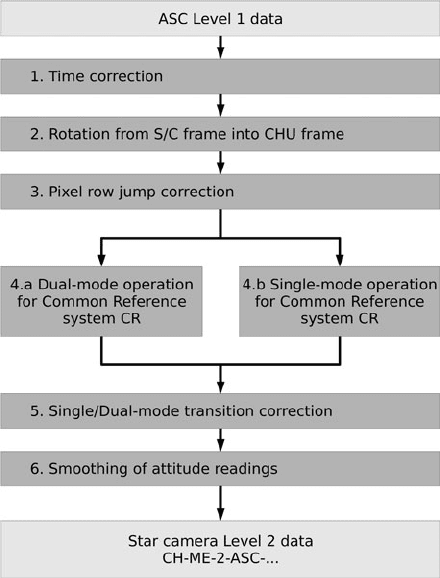
processing to be performed on ground is therefore quite straightforward. Figure 10

presents a schematic ﬂow chart of the ASC data processing steps. It starts again with

the adjustment of the time stamp to the measurement time.

In step 2 the transmitted attitude readings are transformed back from the space-

craft frame into the CHU frame. Step 3 is required for removing artiﬁcial jumps in

the attitude readings. Due to some hardware problems at certain times the readout

of the CCD in the camera does not work properly. In those cases the ﬁrst row of

pixels is skipped. As a result, the internal attitude determination algorithm provides

a biased output. Fortunately, the bias of about 85 arcsec is constant, and can be

removed in the processing. The challenge is to identify the affected readings. An

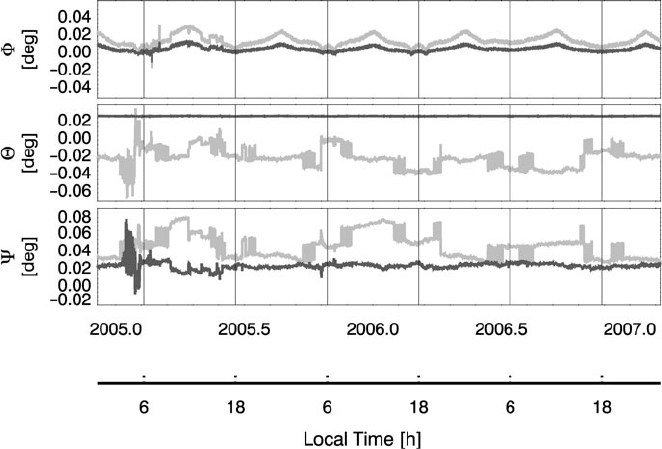
example is given in Fig. 11. The angular differences between CHU1 and CHU2 are

plotted when both attitudes are given in the S/C frame. As expected, there are no

jumps in the rotation around the x axis (roll). In the two other directions, jumps are

evident. Four different states can exist, from both correct attitudes to both biased atti-

tudes. The angle variations after corrections of the attitude jumps are also shown.

Remaining differences between the two independent attitudes are much smaller,

except for the beginning of 2005. Shortly after Christmas 2004 a strong intergalac-

tic gamma burst (Mandea and Balasis, 2006), destroyed a number of CCD pixels.

Only after uploading a new dead-pixel map a reliable attitude determination has

again been possible.

Star trackers have a characteristical anisotropic direction accuracy. While one

can determine the two angles perpendicular to the viewing directions very precisely,

the uncertainty of the rotation angle about the bore-sight is larger by a factor of

492 M. Mandea et al.

Fig. 10 Schematic ﬂow chart for the processing of the Advanced Stellar Compass data. For details

of the processing steps see the text

about 6. To overcome this limitation in step 4a the attitude readings of the two

star trackers are combined, whenever both provide reliable readings. In that case the

uncertainty in the rotation angles can be omitted. A common reference frame (CR) is

deﬁned using exclusively the directions given by the bore-sight of the star cameras.

If these directions are for the camera 1 and 2, respectively, then the reference frame

is calculated by:

=−(Z

+ Z

)/|Z

+ Z

=−(Z

× Z

)/|Z

× Z

= Z

× X

(12)

There are time-intervals, however, when one of the cameras is blinded. In that

case a pre-deﬁned rotation is applied for obtaining the attitude in the CR frame from

the useable camera. Then the quality of the attitude is reduced due to the uncertainty

of the rotation angle. The attitude data are therefore afﬁliated with quality ﬂags

showing on which camera the result is based on. As expected, the transition from

dual head to single head attitude readings is not always smooth. For that reason in

The Earth’s Magnetic Field 493

Fig. 11 Differences between attitudes derived from CHU1 and 2 (both in S/C frame) for 2005–

2007. The grey curve shows the situation before jump correction, and the black curve after

correction

step 5 a ﬁtted linear trend is added to the single head values to ensure a smooth

continuous data series.

A further smoothing is performed in step 6. The CHAMP spacecraft, due to its

large mass, cannot change its attitude rapidly. For that reason, the attitude variations

are constrained, by applying a low-pass ﬁlter. After this processing the ASC Level

2 data are transferred to the ISDC.

2.5 Magnetic Field Data in NEC Frame

An extra demanding task is to rotate the magnetic ﬁeld vector data into a geo-

physically well-deﬁned frame, such as North-East-Center (NEC). Data from several

sources have to be considered for t his transformation. Instruments involved are the

OVM, FGM, ASC and GPS receiver. Only if the readings of all these instruments are

resampled to the same time, given in UTC, they can be combined and transformed.

A time difference of 10 ms can cause an error up to 0.6 nT. On CHAMP all measure-

ment cycles are synchronized by the second-pulse PPS (Precise Positioning Service)

of the GPS receiver, therefore the required timing accuracy of a measurement to a

few milliseconds can be achieved.

A remaining uncertainty of the data in NEC frame comes from the ﬁnite stability

of the optical bench. There is no direct way to check it in space. An indirect approach