Farin G. Curves and Surfaces for CAGD. A Practical Guide

Подождите немного. Документ загружается.

192 Chapter 11 Geometric Continuity

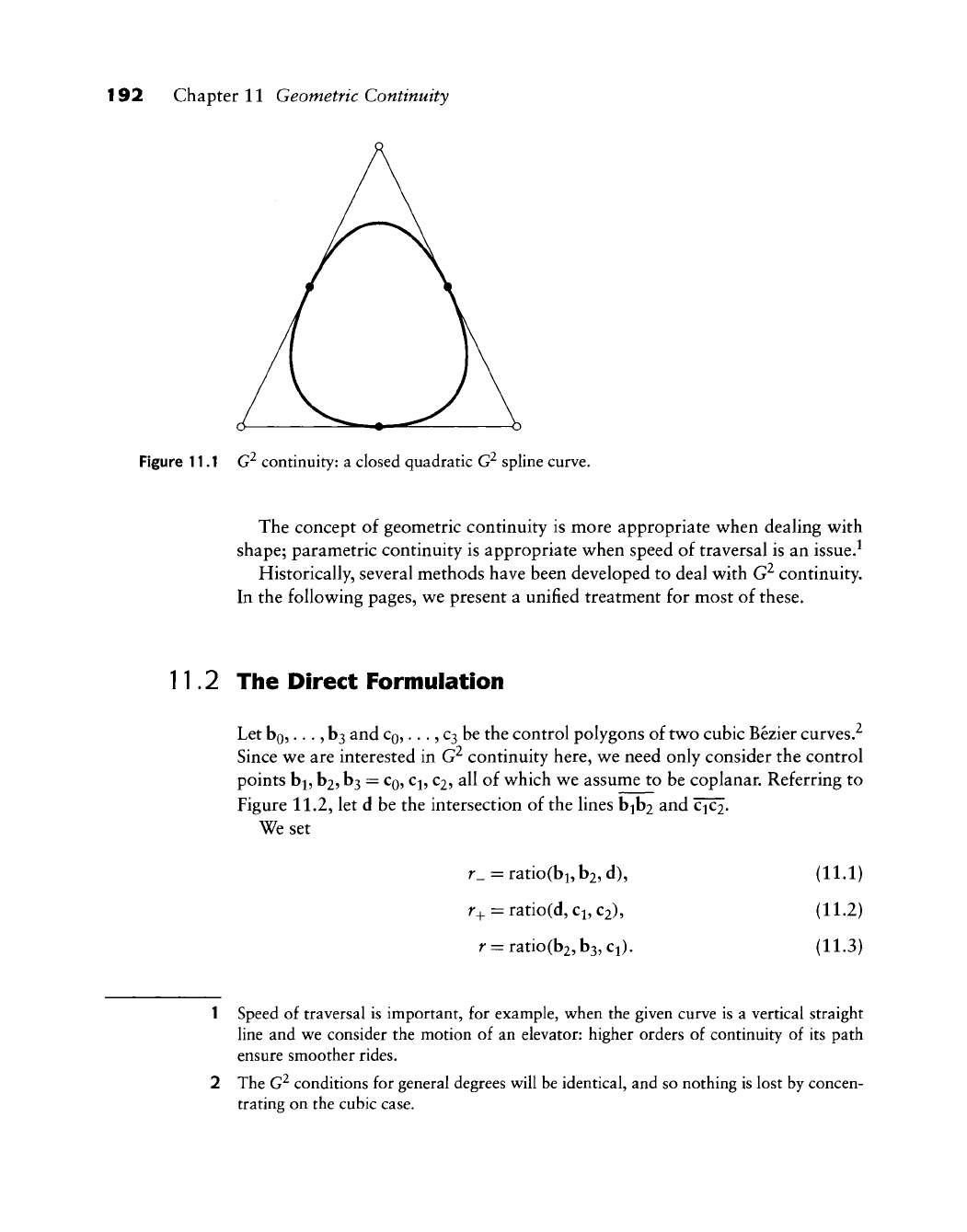
Figure 11.1 G^ continuity: a closed quadratic G^ spline curve.

The concept of geometric continuity is more appropriate when dealing with

shape; parametric continuity is appropriate when speed of traversal is an issue.^

Historically, several methods have been developed to deal with G^ continuity.

In the following pages, we present a unified treatment for most of these.

11.2 The Direct Formulation

Let bo,...,

and

CQ,

...,

be the control polygons of two cubic Bezier curves.-^

Since we are interested in G^ continuity here, we need only consider the control

points bi, b2, b3 =

CQ,

CJ,

C2,

all of which we assume to be coplanar. Referring to

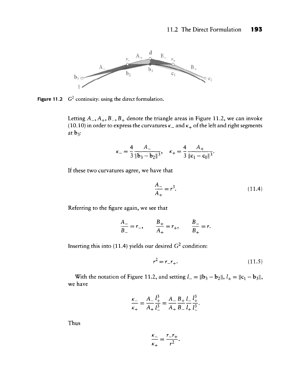
Figure 11.2, let d be the intersection of the lines bib2 and c^.

We set

r_ = ratio(bi,b2,d), (11.1)

r+= ratio(d, Ci,

C2),

(11.2)

r = ratio(b2,b3,Ci). (11.3)

Speed of traversal is important, for example, when the given curve is a vertical straight

line and we consider the motion of an elevator: higher orders of continuity of its path

ensure smoother rides.

The G^ conditions for general degrees will be identical, and so nothing is lost by concen-

trating on the cubic case.

11.2 The Direct Formulation 193

Figure 11.2 G^ continuity: using the direct formulation.

Letting A_,A^,B_,B^ denote the triangle areas in Figure 11.2, we can invoke

(10.10) in order to express the curvatures

and

/c+

of the left and right segments

atbj:

4 A.

4 A,

K,=

3||b3-b2lP' + 3||ci-coll3"

If these two curvatures agree, we have that

Referring to the figure again, we see that

B4-

= r\ (11.4)

T_='-

= r.

A+ -' B^

= r.

Inserting this into (11.4) yields our desired G^ condition:

'-'+'

(11.5)

With the notation of Figure 11.2, and setting /_ = ||b3

—

b2l|, /+ = ||ci

—

b3||,

we have

Thus

r_r.

194 Chapter 11 Geometric Continuity

This is known as Memke's theorem and states that the ratio of left and right

curvatures on any point of a curve is invariant under affine maps. This follows

since we only use affinely invariant ratios in the formulation of K_/K_^.

11.3 The y, Vj and fi Formulations

Using the setting of Section 11.2, we observe that our composite curve could be

made C^ if we introduced a knot sequence with interval lengths A_,

A_^

satisfying

A_/A_^ = r. Using (11.5), we define

We then have

ratio(bi, hi, d) = and ratio(d,

Cj,

C2)

yA+

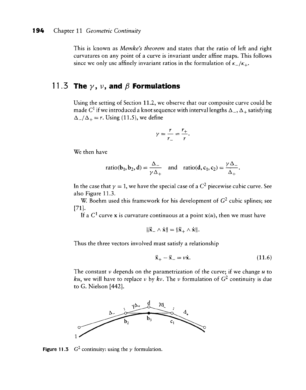
In the case that y = 1, we have the special case of a C^ piecewise cubic curve. See

also Figure 11.3.

W. Boehm used this framework for his development of G^ cubic splines; see

[71].

If a C^ curve x is curvature continuous at a point x(w), then we must have

Thus the three vectors involved must satisfy a relationship

(11.6)

The constant v depends on the parametrization of the curve; if we change u to

ku,

we will have to replace v by ^y. The v formulation of

G'^

continuity is due

to G. Nielson

[442].

Figure 11.3 G^ continuity: using the y formulation.

11.4 G^ Cubic Splines 195

There is a one-to-one relationship between the constants y and v.

„ =

2(^^)1^.

,11.7)

first found by W. Boehm [71].

A similar approach was taken by B. Barsky [40], [47];he uses

Pi = —^ and ^2 =

(11-8)

as the descriptors of G^ continuity and calls them bias and tension, respectively.

Why three or four different formulations for G^ continuity of piecewise cubic

curves? The reason is partly historical, and partly depends on applications. In

fact, the preceding formulations are by no means the only ones—the discussion

of G^ continuity goes back as far as Baer [12], Bezier [59], Geise

[256],

and

Manning

[414].

Applications that aim at constructing surfaces will be better served by ^, y, or

splines. These involve a knot sequence and thus lend themselves to the framework

of tensor product surfaces; see Chapter 16.

Freeform curve design, on the other hand, will benefit more from the direct

formulation since it is linked the closest to the curve geometry. The direct

approach is the most geometric, followed by the y formulation, which needs

a knot sequence. The least geometric are the v and fi formulations; their defining

quantities are not invariant under scaling of the knot sequence.

11.4 C^ Cubic Splines

We start with a control polygon do,..., d^^. In the context of C^ cubic B-splines,

we now needed a knot sequence in order to place the inner Bezier points on the

control polygon legs; the junction points then were fixed by the C^ conditions.

In our case, we have more freedom: we may place the inner Bezier points

anywhere on the control polygon legs; the junction points are then fixed by the

conditions.

To be more precise, consider Figure 11.4. Placing h^j-i ^^ ^^e polygon leg

dj_^i

amounts to picking a number aj (between 0 and 1) and then setting

b3,_2 = (l-aM+M.+l. (11.9)

Similarly, we place h^i_i by picking a number

coj

and setting

196 Chapter 11 Geometric Continuity

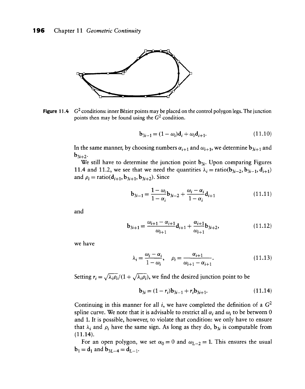
Figure 11.4

conditions; inner Bezier points may

placed on the control polygon

legs.

The junction

points then may be found using the G^ condition.

b3/-i = (1 -

C0i)di

coidi^^,

(11.10)

In the same manner, by choosing numbers aj^i and o^^+i, we determine

h^i-^^

and

We still have to determine the junction point b3/. Upon comparing Figures

11.4 and 11.2, we see that we need the quantities A/ = ratio(b3/_2, b3/_i,

d^_^i)

and

= ratio(d,+i,

^3i-\-h

ba^+i)- Since

b3,-l = i^b3,_2 + ^d,.i (11.11)

—

aj 1

—

and

we have

b3/+l = ^/+1 + b3/+2? (11.12)

= ^, p, = -^i±^. (11.13)

Setting

Yi —

^kiPilil +

y/T~pi)^

we find the desired junction point to be

b3,

= (l-r,)b3,_i + r,b3,+i. (11.14)

Continuing in this manner for all /, we have completed the definition of a G^

spline curve. We note that it is advisable to restrict all a^ and

coi

to be between 0

and 1. It is possible, however, to violate that condition: we only have to ensure

that Xi and pi have the same sign. As long as they do, b3^ is computable from

(11.14).

For an open polygon, we set

Q^Q

= 0 and

(Oi_2

= 1. This ensures the usual

bi = di and h^L-4 = ^L-i-

11.4 G^ Cubic Splines 197

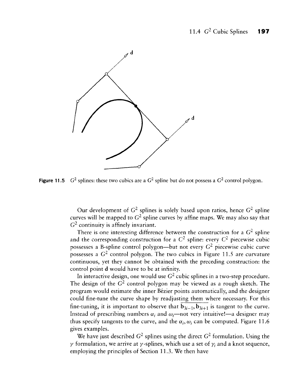
Figure 11.5 G^ splines: these two cubics are a G^ spline but do not possess a G^ control polygon.

Our development of G^ splines is solely based upon ratios, hence G^ spline

curves will be mapped to G^ spline curves by affine maps. We may also say that

continuity is affinely invariant.

There is one interesting difference between the construction for a G spline

and the corresponding construction for a C^ spline: every C^ piecewise cubic

possesses a B-spline control polygon—but not every G^ piecewise cubic curve

possesses a G^ control polygon. The two cubics in Figure 11.5 are curvature

continuous, yet they cannot be obtained with the preceding construction: the

control point d would have to be at infinity.

In interactive design, one would use G^ cubic splines in a two-step procedure.

The design of the G^ control polygon may be viewed as a rough sketch. The

program would estimate the inner Bezier points automatically, and the designer

could fine-tune the curve shape by readjusting them where necessary. For this

fine-tuning, it is important to observe that h^j_i,h^i^i is tangent to the curve.

Instead of prescribing numbers aj and coj—not very intuitive!—a designer may

thus specify tangents to the curve, and the a^,

coj

can be computed. Figure 11.6

gives examples.

We have just described G^ splines using the direct G^ formulation. Using the

y formulation, we arrive at y-splines, which use a set of

and a knot sequence,

employing the principles of Section 11.3. We then have

198 Chapter 11 Geometric Continuity

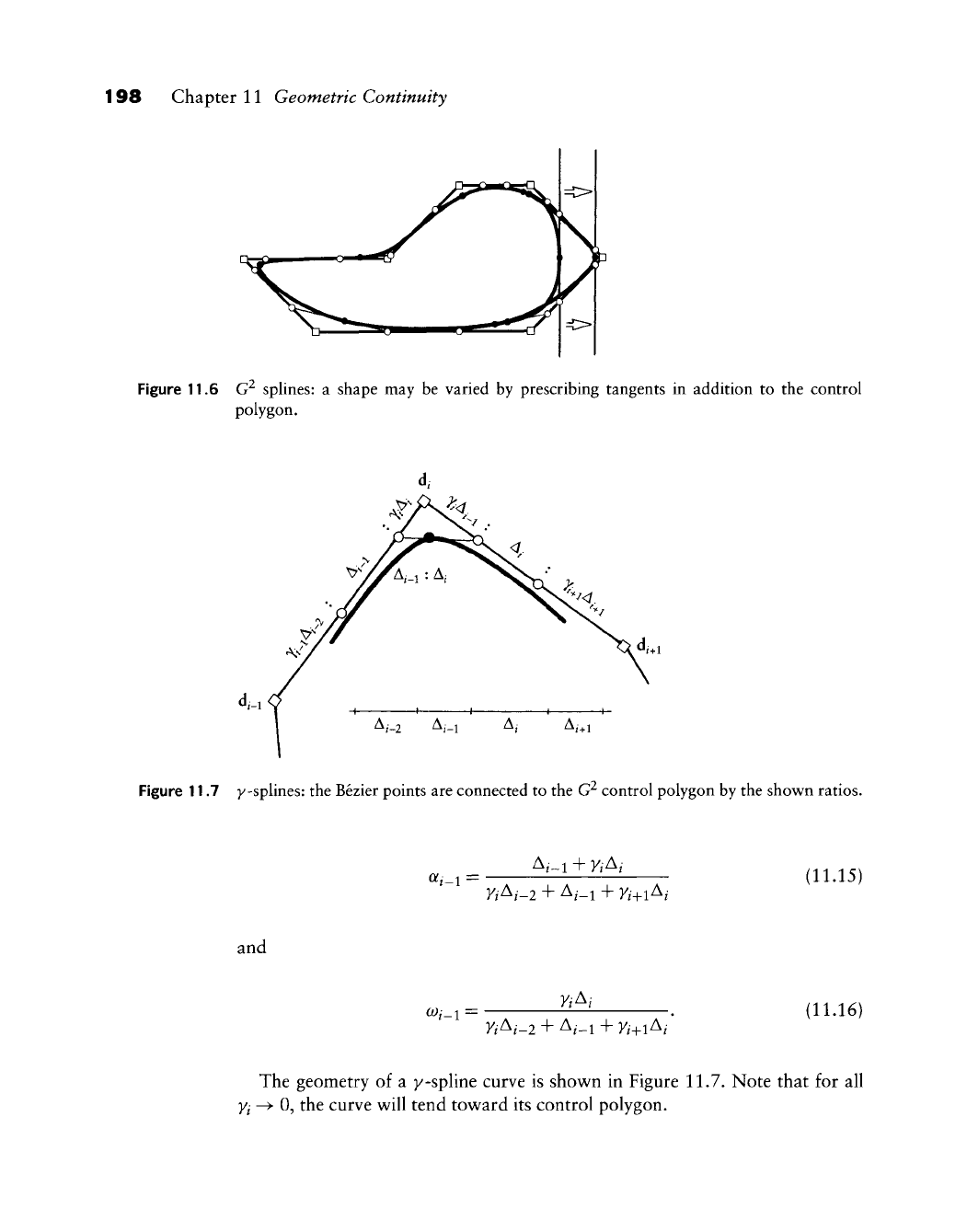
Figure 11.6 G^ splines: a shape may be varied by prescribing tangents in addition to the control

polygon.

A/_2 A,_i A,- A,„i

Figure 11.7 y-splines: the Bezier points are connected to the G^ control polygon by the shown ratios.

a,_l:

A,-i + vAi

VAi-l + A,_i + Yi^i^i

(11.15)

ind

^/-i

vAi

vAi-l + A,_i + Yi^i^i

(11.16)

The geometry of a y-spline curve is shov^n in Figure 11.7. Note that for all

Yl -^ 0, the curve v^ill tend tov^ard its control polygon.

11.5 Interpolating G^ Cubic Splines 199

11.5 Interpolating C^ Cubic Splines

We may also use G^ cubics to interpolate to given data points x^; / = 0,. . ., L.

In the C^ case, we had to supply a knot sequence in addition to the data points.

Now, we have to specify a sequence of pairs a^,

coi.

How to do this effectively is

still an unsolved problem, so let us assume for now that a reasonable sequence

Qfp coi

is given. Setting b3/ = x^, (11.14) yields

d,+i + y/^iOti+A+2,

/•

= 1,..., L - 1. (11.17)

Together with two end conditions, we then have L

— 1

equations for the L + 1

unknowns d^. A suitable end condition is to make d^ a linear combination of

the first three data points: d^ =

WXQ

+ v^\ + wi^i. In our experience, (w,

w) =

(5/6,1/2,

—1/3) has worked well. A similar equation then holds for

dj^^^.

For

the limiting case of aj -> 0 and

coi

-^ 1, the interpolating curve will approach the

polygon formed by the data points. In terms of the y formulation, this spline

type was investigated in

[209].

Nielson [442] derived the G^ interpolating spline from the v formulation.

Assuming that the data points x^ have parameter values

assigned to them, and

using the piecewise cubic Hermite form, the interpolant becomes

xiu) = x^H^ir) + m,A,Hl{r) + A,m,+iH|(r) +

x,_,^Hl(r),

(11.18)

where the

Hj*

are cubic Hermite polynomials from (7.14) and r = (u

—

r^)/A^ is

the local parameter of the interval (r/, r/+i). In (11.18), the

are the known data

points, whereas the m^ are as yet unknown tangent vectors. The interpolant is

supposed to be G^; it is therefore characterized by (11.6), more specifically,

x+(T,)-x_(T,) = y,m, (11.19)

for some constants v^, where m^ = x(r^). The

are constants that can be used to

manipulate the shape of the interpolant; they will be discussed soon. We insert

(11.18) into (11.19) and obtain the linear system

(

A;AX; 1 A;_iAX;\ ^ ^1

^-^i + 'I = A,m,_i + (2A,_i + 2 A, + - A,_iA,y,)m,

A,_i A, / 2

+ A,_im,+i;/=l,...,L-l (11.20)

200 Chapter 11 Geometric Continuity

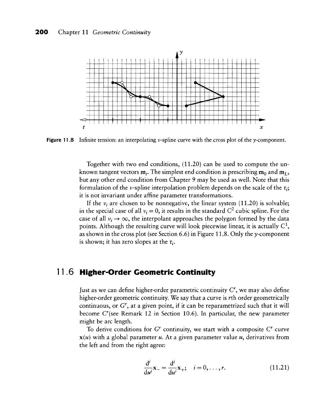
Figure 11.8 Infinite tension: an interpolating y-spline curve with the cross plot of the y-component.

Together with two end conditions, (11.20) can be used to compute the un-

known tangent vectors m^. The simplest end condition is prescribing mo and m^,

but any other end condition from Chapter 9 may be used as well. Note that this

formulation of the y-spline interpolation problem depends on the scale of the r^;

it is not invariant under affine parameter transformations.

If the

are chosen to be nonnegative, the linear system (11.20) is solvable;

in the special case of all

= 0, it results in the standard C^ cubic spline. For the

case of all

-^ oo, the interpolant approaches the polygon formed by the data

points. Although the resulting curve will look piecewise linear, it is actually C^,

as shown in the cross plot (see Section 6,6) in Figure 11.8. Only the y-component

is shown; it has zero slopes at the r^.

11.6 Higher-Order Geometric Continuity

Just as we can define higher-order parametric continuity C^, we may also define

higher-order geometric continuity. We say that a curve is rth order geometrically

continuous, or G^, at a given point, if it can be reparametrized such that it will

become C^(see Remark 12 in Section 10.6). In particular, the new parameter

might be arc length.

To derive conditions for G^ continuity, we start with a composite O curve

x(w) with a global parameter u. At a given parameter value w, derivatives from

the left and from the right agree:

—-x_

= —-x.

au^

:0,...,r.

(11.21)

11.6 Higher-Order Geometric Continuity 201

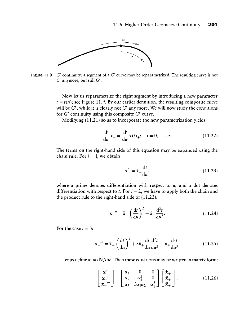
Figure 11.9 G^ continuity: a segment of a

curve may be reparametrized. The resuhing curve is not

C^ anymore, but still G^.

Now let us reparametrize the right segment by introducing a new parameter

t = t{u); see Figure 11.9. By our earlier definition, the resulting composite curve

will be G^, while it is clearly not C any more. We will now study the conditions

for G^ continuity using this composite G^ curve.

Modifying (11.21) so as to incorporate the new parametrization yields:

d' d'

du'

(11.22)

The terms on the right-hand side of this equation may be expanded using the

chain rule. For / = 1, we obtain

X =X

dw'

(11.23)

where a prime denotes differentiation with respect to w, and a dot denotes

differentiation with respect to t. For / = 2, we have to apply both the chain and

the product rule to the right-hand side of (11.23):

„ .. /dty . d^t

(11.24)

For the case / = 3:

X ^'/-x (^\^ 3x —— X

\duj dudu^

dtdh . . dft

dt/3-

(11.25)

Let us define a/ = dH/duK Then these equations may be written in matrix form:

x'_ •

x_"

x_'"

«2

_«3

3o;ia2

0 •

_x+_

(11.26)