Egerton R.F. Electron Energy-Loss Spectroscopy in the Electron Microscope
Подождите немного. Документ загружается.

268 4 Quantitative Analysis of Energy-Loss Data
strongly correlated components of core-loss spectra are the backgrounds to ion-
ization edges but they can be largely removed by taking a derivative of the intensity
(Bonnet and Nuzillard, 2005), so there is some advantage to working with derivative
data.
The principles of ICA are well illustrated by a study by de la Peña et al.
(2011)onaaSn
0.5
Ti
0.5
O
2
nanopowder. They first used EELSLab software (Arenal
et al., 2008) to perform principal component analyis, which is less computer inten-
sive, deals better with noise and avoids problems associated with over-learning
(Hyvärinen et al., 2001). Six principal components were found but as the spec-
tra were not deconvolved to remove plural scattering, some of these components
were suspected to arise from nonlinearity and variations in carbon contamination
thickness. Restricting the analysis to the range above 430 eV reduced the number
of principal components to three, but these appeared to represent a non-physical
mixture of Ti, Sn, and O, making the distribution maps difficult to interpret in
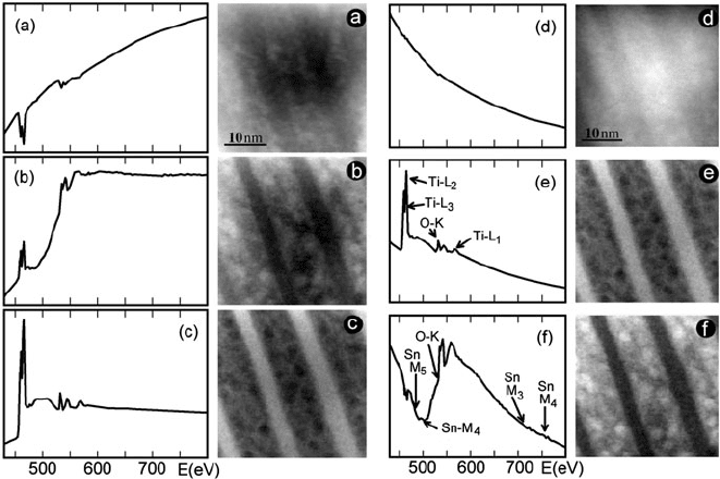
chemical terms; see Fig. 4.15( a–c). Kernel-independent component analysis (Bach
and Jordan, 2002) was then used to extract components that strongly resembled the
spectra of TiO
2
and SnO
2
; see Fig. 4.15(d–f). The fact that the SnO
2
component was
not visible in any of the PCA spectra illustrates the advantage of obtaining signa-
ture spectra for the component oxides, rather than attempting to identify individual
elemental signals (which in this case are compromised because of edge overlap).
Fig. 4.15 (a–c) Three principal components (spectra and images) given by PCA for a Sn
0.5
Ti
0.5
O
2
nanopowder specimen. (d–f) ICA components and distribution maps showing (d) the overall spec-
tral background, (e) rutile-phase TiO
2
,and(f)SnO
2
.FromdelaPeñaetal.(2011), copyright
Elsevier
4.4 Separation of Spectral Components 269
These results demonstrate how ICA can in certain cases transform the principal
components into easily interpretable independent components.
4.4.6 Energy- and Spatial-Difference Techniques
If an energy-loss spectrum is differentiated with respect to energy loss, the
slowly varying background to an ionization edge is largely eliminated. First- or
second-difference spectra can be obtained by digitally filtering conventional spectra
(Zaluzec, 1985; Michel et al., 1993) or by using a spectrum-shifting technique with
a parallel recording spectrometer (Section 2.5.5). These spectra can then be fitted
to energy difference reference spectra, using MLS fitting without the background
term in Eq. (4.73). Because difference spectra are highly sensitive to fine structure
oscillations in intensity, reliable quantification may depend upon the chemical envi-
ronment being similar in the standard and the unknown sample. This condition is
more easily met for metals and biological specimens than for ionic and covalent
materials (Tencé et al., 1995).
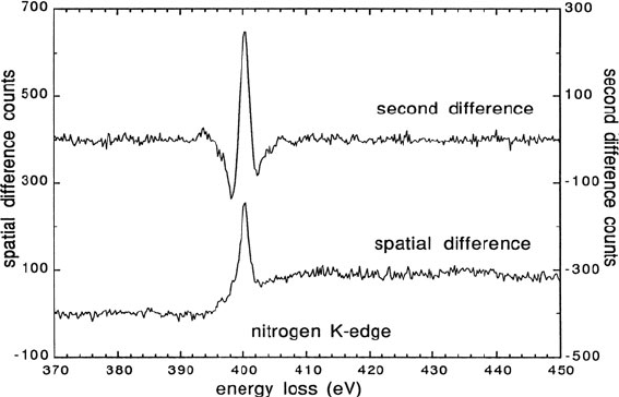
Another way of dealing with the pre-edge background is to record spectra from
a region of interest in the specimen (such as an interface or grain boundary) and
from a nearby “matrix” region. The matrix spectrum (scaled if necessary to allow
for changes in thickness or diffracting conditions) is subtracted from the original
data, yielding a spatial-difference spectrum that represents change in the ionization
edge intensity between the two locations. Because the pre-edge background is
largely eliminated, simple integration can be used for elemental quantification; see
Fig. 4.16.
Fig. 4.16 Spatial difference and second energy difference spectra recorded from a nitrogen-
containing voidite in diamond. The shape of the K-edge (white-line peak followed by a broad
continuum) is consistent with molecular nitrogen. From Müllejans and Bruley (1994), copyright
Elsevier
270 4 Quantitative Analysis of Energy-Loss Data
One advantage of the spatial-difference method is that, provided the changes
in composition are small and the crystal structure is similar in the two locations,
systematic variations in background intensity (due, for example, to extended fine
structures from a preceding edge) are eliminated in the subtraction. Müllejans
and Bruley (1994) have discussed other advantages of this technique in terms of
signal/noise ratio.
A similar spatial-difference procedure can be useful for fine structure stud-
ies (Bruley and Batson, 1989). However, Muller (1999) has argued that bonding
changes at an interface can alter the width of the valence band, producing a change
in local potential and a core-level shift, particularly in 3d transition metals where
the valence states penetrate the atomic core. The core-level shift adds to the differ-
ence spectrum a first-derivative of the edge, which could be mistaken for a white
line. The boundary should be sampled with a sufficiently small probe, so that the
spectrum contains as little intensity as possible from the surrounding volume.
4.5 Elemental Quantification
Because inner-shell binding energies are separated by tens or hundreds of eV, while
chemical shifts (Section 3.7.4) amount to only a few eV, the ionization edges in
an energy-loss spectrum can be used for elemental analysis. The simplest way of
making this analysis quantitative is to integrate the core-loss intensity over an appro-
priate energy window, making allowance for the noncharacteristic background. Such
a procedure is preferable to measuring the height of the edge, which is sensitive to
the near-edge fine structure that depends on the structural and chemical environment
of the ionized atom (Section 3.8). When the element is present in low concentration,
it is difficult to obtain sufficient accuracy in the background extrapolation, so a more
effective procedure is to fit the experimental spectrum in the core-loss region to the
sum of a background and a reference edges, as discussed in Section 4.4.4. In either
case, ionization cross sections for each edge are required.
4.5.1 Integration Method
Incident electrons can undergo elastic, low-loss (plasmon), and core-loss scatter-
ing, making their angular and energy distributions quite complicated. By making
approximations, however, we can obtain simple formulas that are suitable for routine
quantitative analysis.
Assume initially that inner-shell excitation is the only form of scattering in the
specimen. From Eq. (3.94), the integrated intensity of single scattering from shell k
of a selected element, characterized by a mean free path λ
k
and a scattering cross
section σ
k
, would be given by
I
k
1
= I
0
(t/λ
k
) = NI
0
σ
k
(4.62)

4.5 Elemental Quantification 271
I
0
represents the unscattered (zero-loss) intensity and N is the areal density (atoms
per unit area) of the element, equal to the product of its concentration and the spec-
imen thickness. If we record the scattering only up to an angle β and integrate its
intensity over a limited energy range , the coreloss integral is
I
k
1
(β, ) = NI
0
σ
k
(β, ) (4.63)
where σ
k
(β, ) is a “partial” cross section for energy losses within a range of the
ionization threshold and for scattering angles up to β, obtainable from experiment
or calculation (Section 4.5.2).
The effect of elastic scattering is to cause a certain fraction of the electrons to
be intercepted by the angle-limiting aperture. To a first approximation, this fraction
is the same for electrons that cause i nner-shell excitation and those that do not, in
which case I
k
1
(β, ) and I
0
are reduced by the same factor. Therefore the core-loss
integral becomes
I
k
1
(β, ) ≈ NI
0
(β) σ
k
(β, ) (4.64)
where I
0
(β) is the actual (observed) zero-loss intensity. Equation (4.64) applies to a
core-loss edge from which plural (core-loss + plasmon) scattering has been removed
by deconvolution.
If we now i nclude valence electron (plasmon) excitation as a contribution to the
spectrum, its effect is to redistribute intensity toward higher energy loss, away from
the zero-loss peak and away from the ionization threshold. Not all of this scattering
falls within the core-loss integration window, but to a first approximation the fraction
that is included will be the same as the fraction that falls within an energy window
of equal width in the low-loss region. If so, the core-loss integral (including plural
scattering) is given by
I
k
(β, ) ≈ NI(β, ) σ
k
(β, ) (4.65)
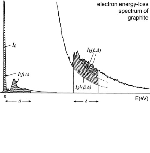
where I(β,) is the low-loss intensity integrated up to an energy-loss ;see
Fig. 4.17.
Although Eqs. (4.64) and (4.65) allow measurement of the absolute areal density
N of a given element, an atomic ratio of two elements (a and b) is more commonly
required. Provided the same integration window is used for both edges, Eq. (4.65)
gives
N
a
N
b
=
I
ka
(β, )
I
jb
(β, )
σ
jb
(β, )
σ
ka
(β, )
(4.66)
The shell index can be different for the two edges (j = k); K-edges are suitable for
very light elements (Z < 15) and L-orM-edges for elements of higher atomic num-
ber. However, our approximate treatment of plural scattering will be more accurate if
the two edges have similar shape. If plural scattering is removed from the spectrum
by deconvolution, Eq. (4.64) leads to
272 4 Quantitative Analysis of Energy-Loss Data
Fig. 4.17 Energy-loss spectrum showing the low-loss region and (with change in intensity scale)
a single ionization edge. The cross-hatched area represents electrons that have undergone both
core-loss and low-loss scattering
N
a
N
b
=
I
1
ka
(β,
a
)
I
1
jb
(β,
b
)
σ
jb
(β,
b
)
σ
ka
(β,
a
)
(4.67)
A different energy window (
a
=
b
) can now be used for each edge, larger values
being more suitable at higher energy loss where the spectrum is noisier and the
edges representing different elements are spaced further apart.
Several authors have tested the accuracy of these equations for thin specimens.
Approximating the low-loss spectrum by sharp peaks at multiples of a plasmon
energy E
p
, Stephens (1980) concluded that the approximate treatment of plural
scattering inherent in Eq. (4.65) will lead to an error in N of between 3 and 10%
(dependent on E
k
)fort/λ
p
= 0.5 and /E
p
= 5. The error would be some fraction
of this when evaluating elemental ratios. Systematic error arising from the angular
approximation inherent in Eq. (4.64) was estimated to be of the order of 1% for a
20-nm amorphous carbon film but considerably larger for polycrystalline or single-
crystal specimens if a strong diffraction ring (or spot) occurs just inside or outside
the collection aperture (Egerton, 1978a).
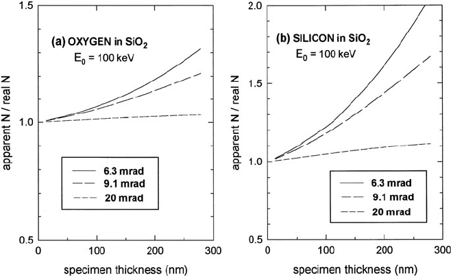
As specimen thickness increases, the higher probability of elastic and plural
scattering causes Eqs. (4.64), (4.65), (4.66), and (4.67) to become less accurate.
Elemental ratios given by Eq. (4.66)or(4.67) were found to change when t/λ
exceeded approximately 0.5 (Zaluzec, 1983). This variation was attributed to the
effect of elastic scattering and has been modeled for amorphous materials of known
composition, using an elastic scattering angular distribution given by the Lenz
model (Cheng and Egerton, 1993, Su et al., 1995). Correction factors can be evalu-
ated for specimens of unknown composition, based on additional measurements of
the low-loss spectrum at several collection angles (Wong and Egerton, 1995). Such
4.5 Elemental Quantification 273
Fig. 4.18 Factor by which the area density obtained from Eq. (4.64) should be divided to correct
for elastic scattering, in the case of (a) the oxygen K-edge and (b) the silicon K-edge in amorphous
silicon dioxide. From Cheng and Egerton (1993), copyright Elsevier
correction becomes significant at specimen thicknesses above 100 nm, particularly
for higher edge energy and small collection angle; see Fig. 4.18.
Precise correction for elastic scattering in crystalline specimens is a difficult task;
it would require the measurement of intensity in the diffraction plane or a knowledge
of the crystal structure, orientation, and thickness of the specimen. The situation in
single-crystal specimens is further complicated by the existence of channeling and
blocking effects; see Sections 3.1.4 and 5.6.
4.5.2 Calculation of Partial Cross Sections
If the core-loss intensity is integrated over an energy window that is wide enough
to include most of the fine structure oscillations, the corresponding cross section
σ
k
(β, ) should be little affected by the chemical environment of the excited atom,
and can therefore be calculated using an atomic model. Weng and Rez (1988)
estimated that atomic cross sections are accurate to within 5% for >20eV.
The simplest atomic model is based on the hydrogenic approximation, for
which the generalized oscillator strength (GOS) is available in analytic form; see
Section 3.4.1. Computation is therefore rapid and requires only the atomic num-
ber Z, edge energy E
K
, integration range , angular range β, and incident electron
energy E
0
as inputs. Computer programs for the calculation of K- and L-shell cross
sections are described in Appendix B.

274 4 Quantitative Analysis of Energy-Loss Data
More sophisticated procedures, such as the Hartree–Slater method, involve more
extensive computation and a greater knowledge of atomic properties. However, the
resulting GOS can be parameterized as a function of the energy and wave number
q and the resulting values integrated according to Eqs. (3.151) and (3.157) to yield
a cross section. Parameterization can also take account of EELS experiments and
(for small q) x-ray absorption measurements. A program giving K-, L-, M-, N-, and
O-shell cross sections, valid for small β, is described in Appendix B.
A completely experimental approach to quantification is also possible, the sensi-
tivity factor for a given edge being obtained by measurements on standards (Malis
and Titchmarsh, 1986; Hofer, 1987; Hofer et al., 1988). If these measurements are
made in the same microscope and under the same experimental conditions as used
for the unknown specimen, the procedure should be relatively insensitive to the
chromatic aberration of prespectrometer lenses (Section 2.3.3) and imperfect knowl-
edge of the collection angle and incident electron energy. It is analogous to the
k-factor procedure used in thin-film EDX microanalysis. An experimentally deter-
mined k-factor can be converted to a dipole oscillator strength f() that depends only
on the integration range , allowing partial cross sections to be calculated for any
incident electron energy and collection angle within the dipole region. Alternatively,
the generalized oscillator strengths obtained from Hartree–Slater cross sections can
be parameterized (as a function of energy loss and scattering angle) and used to
calculate σ
k
(β,) for a wide range of Z, E
0
, , and β, as in the Gatan DM software.
4.5.3 Correction for Incident Beam Convergence
Equations (4.64), (4.65), (4.66), and (4.67) assume that the angular spread of the
incident beam is small in comparison with the collection semi-angle β, a condi-
tion that applies to broad beam TEM illumination but easily violated if the incident
electrons are focused into a fine probe of large convergence semi-angle α.For
such a probe, the angular distribution of the core-loss intensity dI
k
/d can be cal-
culated as a vector convolution of the incident electron intensity dI/d and the
inner-shell scattering dσ
k
/d. Taking the latter to be a Lorentzian function of width
θ
E
= E/(γ m
0
v), with E ≈ E
k
+/2, we obtain
dI
k
d
∝
α
θ
0
=0
2π
φ=0
dI
d
1
θ
2
k
+θ
2
E
θ
0
dθ
0
dφ (4.68)
where θ
k
2
= θ
2
+θ
0
2
−2θθ
0
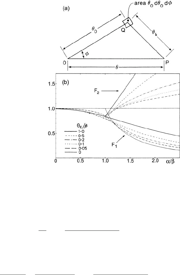
cos ϕ; see Fig. 4.19a. The core-loss intensity passing
through a collection aperture of semi-angle β is then
I
k
(α, β, θ
E
) =
β
0
dI
k
d
2πθdθ (4.69)
4.5 Elemental Quantification 275
Fig. 4.19 (a) Calculation of
the core-loss intensity at P (an
angular distance θ from the
optic axis) due to electrons at
Q (polar coordinates θ
0
and φ). The angle of inelastic
scattering is θ
k
.
(b) Convergence-correction
factors F
1
and F
2
, plotted as a
function of the convergence
semi-angle α of the incident
beam, for different values of
the characeristic scattering
angle θ
E
. Note that for α < β,
the correction factor
(F
1
= F
2
) first decreases and
then increases with increasing
θ
E
. From Egerton and Wang
(1990), copyright Elsevier
If it is true that the incident intensity per unit solid angle remains constant up to a
cutoff angle α, the double integral of Eq. (4.68) can be solved analytically (Craven
et al., 1981), giving
dI
k
d
∝ ln
ψ
2
+(ψ
4
+4θ
2
θ
2
E
)
1/2
2θ
2
E
(4.70)
where ψ
2
= α
2
+θ
E
2
−θ
2
. Combining the previous three equations yields
F
1
=
I
k
(α, β, )
I
k
(0, β, )
=
2/α
2
ln
)
1 +
(
β/θ
E
)
2
*
β
0
ln
ψ
2
+(ψ
4
+4θ
2
θ
2
E
)
1/2
2θ
2
E
θdθ (4.71)
F
1
is a factor (<1) representing reduction in the measured core-loss intensity due to
incident beam convergence. Scheinfein and Isaacson (1984) showed that the integral
in Eq. (4.71) can be expressed analytically, and their expression is used to evaluate
F
1
in the program CONCOR2 listed in Appendix B. Because F
1
depends to some

276 4 Quantitative Analysis of Energy-Loss Data
degree on θ
E
(see Fig. 4.19), the convergence correction is different for each ioniza-
tion edge. When using Eq. (4.66)or(4.67) to obtain an elemental ratio, the effect of
beam convergence is included by multiplying the right-hand side by F
1b
/F
1a
.
To obtain a correction factor for absolute quantification, we need to consider the
effect of beam convergence on the low-loss intensity. Since θ
E
/β << 1 for valence
electron scattering, the corresponding factor F
1
is close to 1 provided α < β (see
Fig. 4.19). If α > β, the recorded low-loss intensity is approximately proportional
to the area of the convergent-beam disk that falls within to the collection aperture,
so Eq. (4.65) becomes
I
k
(α, β, ) ≈ F
2
N σ
k
(β, )I(α, β, ) (4.72)
where F
2
≈ F
1
for α ≤ β and F
2
≈ (α/β)
2
F
1
for α ≥ β; see Fig. 4.19b.
Alternatively, the effect of incident beam convergence can be expressed in terms
of an effective collection angle β
∗
that differs from β by an amount dependent on
α and the edge energy. To allow for the possibility of absolute quantification (or
thickness measurement by the log-ratio method, Section 5.1.1), we should take
I
k
(α, β, ) = F
2
I
k
(β, ) = I
k
(β
∗
, ), (4.73)
in which case β
∗
>βfor α>β.
Kohl (1985) has pointed out that incident beam convergence can be included in an
effective cross section σ
k
(α, β, ), which could incorporate a non-Lorentzian angu-
lar dependence at high angles, although for large collection angle the convergence
correction is small anyway. Because the angular dependence of the incident beam
intensity dI/d is usually unknown, and almost certainly deviates from a rectangular
function, any convergence correction is likely to be approximate.
4.5.4 Quantification from MLS Fitting
The coefficients B
n
obtained from Eq. (4.61a) by multiple least-squares fitting can
be used to derive atomic ratios of the elements involved. For ultrathin specimens,
or if deconvolution has removed plural scattering, the reference spectra S
n
(E) can
be calculated differential cross sections (Steele et al., 1985), in which case each
coefficient B
i
is the product of the zero-loss intensity and the areal density of the
appropriate element.
More usually, each S
i
(E) is measured on an aribitary intensity scale from a stan-
dard specimen containing the appropriate element, in which case the atomic ratio of
any two elements (a and b) is obtained from
N
a
N
b
=
B
a
B
b
I
ka
(
β,
)
I
kb
(
β,
)
σ
kb
(
β,
)
σ
ka
(
β,
)
(4.74)
4.6 Analysis of Extended Energy-Loss Fine Structure 277
where I
ka
(β, ) and I
kb
(β, ) are integrals (over some convenient integration range
) of the core-loss spectra of the appropriate standards, σ
ka
(β, ) and σ
kb
(β, )
being the partial cross sections evaluated for the appropriate collection angle β,
allowing for incident beam convergence if necessary (Section 4.5.3).
If the analyzed specimen is appreciably thicker than the standard, the reference
edge may need to be convolved with the low-loss region of the analyzed speci-
men, to make allowance for plural scattering. If the region just above the ionization
edge contains prominent fine structure that is sensitive to the chemical environment
of each element (Section 3.8), this region may have to be excluded from the fit-
ting, especially if the chemical environments of the specimens are very different.
Alternatively, fitting to an atomic model in the near-edge region might yield valu-
able density of states information (Verbeeck et al., 2006). For good accuracy or
weak edges, the importance of allowing for correlated (fixed pattern) noise of the
electron detector has been emphasized (Verbeeck and Bertoni, 2008). Atomic-ratio
accuracies better than 3% and precisions better than 10% have been obtained using
test compounds (Bertoni and Verbeeck, 2008).
Riegler and Kothleitner (2010) have analyzed chromium concentrations down to
0.1% by using MLS fitting and have derived a formula for the minimum atomic
fraction detectable using this procedure; see Section 5.5.4.
4.6 Analysis of Extended Energy-Loss Fine Structure
As discussed in Section 3.9, the EXELFS modulations that extend over some hun-
dreds of eV beyond an ionization edge can be analyzed to provide the distances
of near-neighbor atoms from an atom of known chemical species in a TEM spec-
imen. In favorable circumstances, coordination numbers, bond angles, and degree
of atomic disorder are also measurable. This information is of particular value in
the case of multielement amorphous materials, where diffraction techniques cannot
distinguish the elastic scattering from different elements.
4.6.1 Fourier Transform Method
Following the original EXAFS procedure ( Sayers et al., 1971), the radial distribution
function (RDF) is obtained as a Fourier transform of the experimental EXELFS data
(Kincaid et al., 1978; Johnson et al., 1981a; Leapman et al., 1981; Stephens and
Brown, 1981; Bourdillon et al., 1984). The essential steps involved are as follows.
4.6.1.1 Background Subtraction and Deconvolution
Unless the specimen is very thin (<10 nm, for 100-keV electrons), plural scattering
beyond the edge is first removed by deconvolution. If the Fourier ratio technique is
used (Section 4.3.2), the pre-edge background is subtracted prior to deconvolution;