Durst F. Fluid Mechanics: An Introduction to the Theory of Fluid Flows

Подождите немного. Документ загружается.

24 2 Mathematical Basics

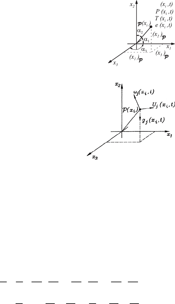
Fig. 2.4 Scalar ﬁelds assign a scalar to each point in

the space and as a function of time

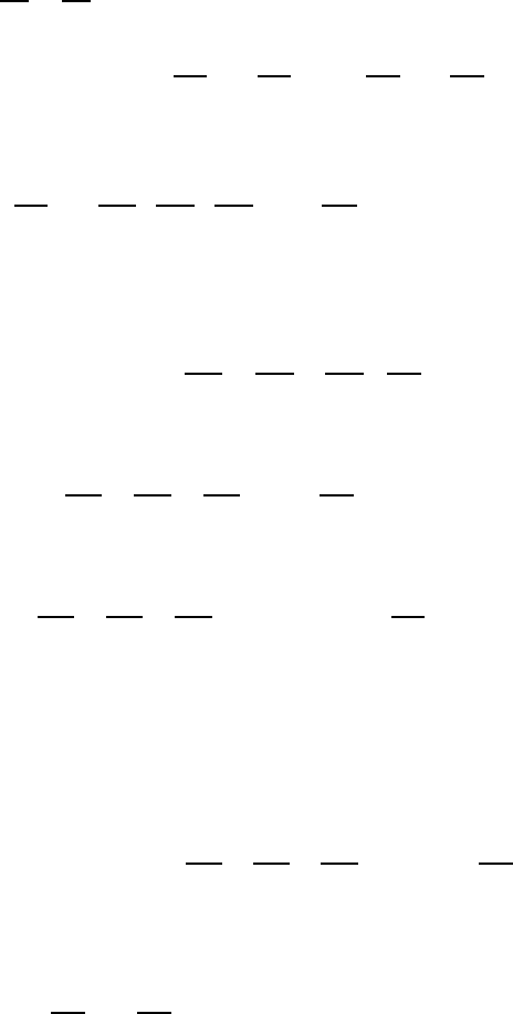
Fig. 2.5 Vector ﬁelds assign vectors to each

point in the space as functions of time

P(x

)attimet.Itrepresentsthej-momentum transport acting in the x

di-

rection. Further, 

,t) represents the ﬂuid element deformation depending

on the gradients of the velocity ﬁeld at the location P(x

)attimet.

The properties introduced as ﬁeld variables into the above considerations

represented tensors of zero order (scalars), tensors of ﬁrst order (vectors) and

tensors of second order. They are employed in ﬂuid mechanics to describe

ﬂuid ﬂows and the corresponding ﬂuid description is usually attributed to

Euler (1707–1783). In this description, all quantities considered in the repre-

sentations of ﬂuid mechanics are dealt with as functions of space and time.

Mathematical operations such as addition, subtraction, division, multiplica-

tion, diﬀerentiation and integration, that are applied to these quantities, are

subject to the known laws of mathematics.

The diﬀerentiation of a scalar ﬁeld, for example the density ρ(x

,t), gives

dρ

∂ρ

∂t

∂ρ

∂x





∂ρ

∂x





∂ρ

∂x





(2.32)

∂ρ

∂t



i=1



∂ρ

∂x





∂ρ

∂t



∂ρ

∂x





In the last term, the summation symbol



i=1

was omitted and the “Einstein’s

summation convention” was employed, according to which the double index

2.5 Field Variables and Mathematical Operations 25

i in



∂ρ

∂x





prescribes a summation over three terms i =1, 2, 3, i.e.:



i=1



∂ρ

∂x







∂ρ

∂x





(2.33)

The diﬀerentiation of vectors is given by the following expressions:





⇒

,i=1, 2, 3 (2.34)

i.e. each component of the vector is included in the diﬀerentiation. As the

considered velocity vector depends on the space location x

and the time t,

the following diﬀerentiation law holds:

∂U

∂t

∂U

∂x





(2.35)

When one applies the Nabla or Del operator:

∇ =



∂

∂x

∂

∂x

∂

∂x





∂

∂x



,i=1, 2, 3 (2.36)

on a scalar ﬁeld quantity, a vector results:

∇a =



∂a

∂x

∂a

∂x

∂a

∂x



=grada =



∂a

∂x



,i=1, 2, 3 (2.37)

This shows that the Nabla or Del operator ∇ results in a vector ﬁeld deduced

from the gradient ﬁeld. The diﬀerent components of the resulting vector are

formed from the prevailing partial diﬀerentiations of the scalar ﬁeld in the

directions x

The scalar product of the ∇ operator with a vector yields a scalar quantity,

i.e. when (∇·) applied to a vector quantity results in:

∇·a =

∂a

∂x

∂a

∂x

∂a

∂x

=diva =

∂a

∂x

(2.38)

Here, in ∂a

/∂x

the subscript i again indicates summation over all three

terms, i.e.



i=1

∂a

∂x

=⇒

∂a

∂x

(Einstein’s summation convention) (2.39)

The vector product of the ∇ operator with the vector a yields correspondingly

∇×a =



∂/∂x



⎧

⎨

⎩

∂a

/∂x

− ∂a

/∂x

∂a

/∂x

− ∂a

/∂x

∂a

/∂x

− ∂a

/∂x

⎫

⎬

⎭

=rota (2.40)

26 2 Mathematical Basics

∇×a =rota = −

ijk

∂a

∂x

= 

ijk

∂a

∂x

(2.41)

The Levi–Civita symbol 

ijk

is also called the alternating unit tensor and is

deﬁned as follows:



ijk



0 : if two of the three indices are equal

+1 : if ijk = 123, 231 or 312

−1:if ijk = 132, 213 or 321

(2.42)

Concerning the above-mentioned products of the ∇ operator, the distributive

law holds, but not the commutative and associative laws.

If one applies the ∇ operator to the gradient ﬁeld of a scalar function, the

Laplace operator ∇

(alternative notation ∆) results. When applied to a,the

result can be written as follows:

∇

a =(∇·∇)a =

∂

∂x

∂

∂x

∂

∂x

∂

∂x

(2.43)

The Laplace operator can also be applied to vector ﬁelds, i.e. to the compo-

nents of the vector:

∇

U =

⎛

⎜

⎝

∇

⎞

⎟

⎠

⎛

⎜

⎝

∂

/∂x

∂

/∂x

∂

/∂x

∂

/∂x

∂

/∂x

∂

/∂x

∂

/∂x

∂

/∂x

∂

/∂x

⎞

⎟

⎠

(2.44)

2.6 Substantial Quantities and Substantial Derivative

A further approach to describing ﬂuid mechanics processes is to derive the

basic equations in terms of substantial quantities. This approach is generally

named after Lagrange (1736–1813) and is based on considerations of proper-

ties of ﬂuid elements. The state quantities of a ﬂuid element  such as the

density ρ



, the pressure P



, the temperature T



and the energy e



are em-

ployed for the derivation of the laws of ﬂuid motion. If one wants to measure

or describe these properties of a ﬂuid element in a ﬁeld, one has to move with

the element, i.e. one has to follow the path of the element:

)

,T

=(x

)

,0

)



dt (2.45)

As the path of a ﬂuid element is only a function of time t and an initial space

coordinate (x

)

,0

, the substantial quantities, i.e. the thermodynamic state

quantities of a ﬂuid element can also only be functions of time.

2.7 Gradient, Divergence, Rotation and Laplace Operators 27

Thus the total diﬀerentials of all substantial quantities can be formulated

as follows, with reference to (2.35):



∂a

∂t

∂a

∂x







, where







=(U

)



(2.46)

The quantity speciﬁed with (dx

/dt)



indicates the change of position of a

ﬂuid element  with time, i.e. the substantial velocity of a ﬂuid element.

If a ﬂuid element is positioned at time t at location x

,then(U

)



= U

results and from this arises the ﬁnal equation of the substantial derivative of

aﬁeldvariableDa/Dt:



∂a

∂t

+ U

∂a

∂x

(2.47)

This equation results also from the identity relationship. This states, for a

representation of a ﬂuid ﬂow in two diﬀerent ways, without contradiction,

that the following equality of Euler and Lagrange variables holds:



(t)=a(x

,t)if(x

)



= x

at time t

From this one can derive



∂a

∂t

+(U

)



∂a

∂x

∂a

∂t

+ U

∂a

∂x

(2.48)

From (2.47), it can be seen that the operator

(= substantial derivative)

can be written as follows:

∂

∂t

+ U

∂

∂x

∂

∂t

+(U ·∇) (2.49)

This operator can be applied to ﬁeld variables and is very important for the

subsequent derivations of the basic equations of ﬂuid mechanics, as it permits

the formulation of the basic equations in Lagrange variables and in a second

step the subsequent transformation of all terms in this equation into Euler

variables. In this ﬁnal form, i.e. expressed in Euler variables, the equations

are suited for the solution of practical ﬂow problems.

2.7 Gradient, Divergence, Rotation

and Laplace Operators

a(x

,t) represents a scalar ﬁeld, i.e. it is deﬁned or given as a function of space

and time. The gradient ﬁeld of the scalar ‘a’ can be assigned the following

components at each point in a space:

28 2 Mathematical Basics

a(x

,t)=⇒



∂a

∂x



=grad(a)=

⎧

⎨

⎩

∂a/∂x

⎫

⎬

⎭

;grad(a)=f(x

,t) (2.50)

Thus the operator grad( ) is deﬁned as follows:

grad() =



∂()

∂x





∂()

∂x

∂()

∂x

∂()

∂x



(2.51)

i.e. grad(a) is a vector ﬁeld, whose components are marked by the index i.

The grad(a) vectors exhibit directions which are perpendicular to the lines

of a = constant of the considered scalar ﬁeld, i.e. perpendicular to a(x

,t)=

constant.

Furthermore, the Laplace operator can be assigned to each scalar ﬁeld

a(x

,t) ⇒ ∆a(x

,t) (J.S. Laplace (1749–1827)). Here, ∆a(x

,t) is a scalar

ﬁeld, e.g. to each space point the quantity ∆(a)isassigned

∆a(x

,t)=

∂

∂x

∂

∂x

∂

∂x

∂

∂x

(2.52)

Employing the previously deﬁned divergence operator, the following equation

results:

∆a(x

,t) = div(grad a)=div



∂a

∂x



∂

∂x

∂

∂x

(2.53)

For the mathematical treatment of ﬂow problems, there are other mathemat-

ical operators of importance, in addition to the operators div( ) and rot( ) =

curl( ) that are applicable to vector ﬁelds such as U (x

,t) and are deﬁned as

follows:

div (U (x

,t)) =

∂U

∂x

∂U

∂x

∂U

∂x

∂U

∂x

(2.54)

and

rot U(x

,t)=

ijk

∂U

∂x

⎧

⎨

⎩

∂U

/∂x

− ∂U

/∂x

∂U

/∂x

− ∂U

/∂x

∂U

/∂x

− ∂U

/∂x

⎫

⎬

⎭

(2.55)

Here, div U is a scalar ﬁeld and rot or curl U are vector ﬁelds. When U is a

velocity ﬁeld, the value of div U describes the temporal change of the volume

δV



of a ﬂuid element with constant mass δm



, i.e.

div (U )=

∂U

∂x

δV



d(δV



)

(2.56)

If the density ρ = constant is included, div(ρU ) implies a mass density source

at the point x

at time t. Correspondingly, rot (U)orcurl(U )representthe

vortex density of the velocity ﬁeld at the point x

at time t.Ifcurl(U)=0,

a ﬂuid element at the point x

,andattimet, experiences no contribution

2.8 Line, Surface and Volume Integrals 29

to its rotation by the velocity ﬁeld. For rot (U) =0attimet and at point

, a ﬂuid element consequently experiences, at the corresponding point, a

contribution to its rotational motion.

In summary, the operators described above can be formulated as follows:

grad(a)=



∂a

∂x



= ∇a (2.57)

div (U )=∇·U

∂U

∂x

(2.58)

∆a = ∇

a = ∇·∇a =

∂

∂x



∂a

∂x



∂

∂x

(2.59)

rot (U )=∇×U = 

ijk

∂U

∂x

(2.60)

These operators will be employed for the derivation of the basic equations of

ﬂuid mechanics and also when dealing with ﬂow problems.

2.8 Line, Surface and Volume Integrals

The line integral of a scalar function a(x

,t) along a line S is deﬁned as

follows:

(t)=

a dS =

a(x

,t)dS with x

∈ S (2.61)

Line integrals of this kind are required in ﬂuid mechanics to deﬁne the position

of the “center of gravity” of a line. Their computation is carried out in three

stepsasfollowsfort = constant:

1. The viewed curve is parameterized:

S : s(γ)={s

(γ)}

,α≤ γ ≤ β (2.62)

2. The arched element ds is deﬁned by diﬀerentiation:

ds =



(γ)

dγ



dγ =



(γ)

dγ



dγ (2.63)

3. The computation of the deﬁned integral from γ = α to γ = β:

a(s

(γ))



dγ



dγ ; I

(2.64)

The application of the above steps for the computation of the deﬁned integral

leads for a = 1 to the length of the considered curve s(γ) between γ = α and

γ = β.

30 2 Mathematical Basics

Analogous to the above considerations, the integration of a vector ﬁeld

along a curve can be carried out in the following way:

(t)=

· ds

(γ))

(γ)

dγ

dγ at time t (2.65)

Computations of the work done in the ﬁelds of forces, the circulation

of mass and momentum ﬂow in the case of two-dimensional ﬂow ﬁelds are

eﬀected via such deﬁned integrations of vector ﬁelds along space lines.

Analogous to the integrals along lines or along line segments, space inte-

grals for scalar and vectors can also be deﬁned and computed according to

the following computation rules:

(t)=

a dF at time t (2.66)

If F is the surface area of a considered ﬂuid element and a(x

,t) a scalar ﬁeld,

that is continuous on the surface, the above integral as the surface integral is

named from a to F . The surface-averaged value of a is computed as follows:

˜a =

a dF

(surface mean value) (2.67)

For the surface integral of a vector ﬁeld holds that

(t)=

dF at time t (2.68)

For the case a

= U

, i.e. the execution of a surface integration over the veloc-

ity ﬁeld, an integral value is obtained that corresponds to the instantaneous

volume ﬂow through the surface F :

Q(t)=

(volume ﬂow through F at time t) (2.69)

Analogously, the mass ﬂow through F is computed by

M(t)=

ρU

(mass ﬂow through F at time t) (2.70)

The mean mass ﬂow density is given by

˙m(t)=

ρU

(2.71)

2.9 Integral Laws of Stokes and Gauss 31

The above integrations can be extended to volume integrals, which again

can be applied to scalar and vector ﬁelds. If V designates the volume of a

regular ﬁeld and a(x

,t) a steady scalar ﬁeld (occupation function) given in

this space, the total occupancy of the space is computed as follows:

(t)=

a dV (total occupancy of V through a at time t) (2.72)

The mass of a regular space with the density distribution ρ(x

,t)resultsin

the following triple integral of the density distribution ρ(x

,t):



M(t)=

ρ(x

,t)dx

(2.73)

Here, variables with %and &symbols indicate surface- and volume-averaged

quantities in this chapter of the book.

For the practical implementation of surface and volume integrations, it is

often advantageous to employ the laws of Guldin:

1. Law of Guldin (1577–1643): The surface area of a body with rotational

symmetry is given by

2π · r(s)ds,withds denoting an arc element of

the plane curve s generating the body and r(s) denoting the distance of

ds from the axis of rotation.

2. Law of Guldin (1577–1643): The volume of a body with rotational sym-

metry is given by

2π · r

(F ) · dF ,withdF denoting an area element

oftheareaenclosedbytheplanecurves generating the body and r

(F )

denoting the distance of dF from the axis of rotation.

2.9 Integral Laws of Stokes and Gauss

The integral law named after Stokes (1819–1903) reads

(

a · ds =

rot a · dF (2.74)

which means that the line integral of a vector a over the entire edge line of

a surface is equal to the surface integral of the corresponding rotation of the

vector quantity over the surface. Thus the integral law of Stokes represents

a generalization of Green’s law (1793–1841), which was formulated for plane

surfaces, i.e. for “spatial areas”. If one stretches two diﬀerent surfaces over a

boundary of surface S, Stokes’ law gives

rot a · dF =

rot a · dF (2.75)

32 2 Mathematical Basics

where S is equal to the stretching quantities of O

and O

. If one introduces

by Γ =

)

Uds the term of circulation of a vector ﬁeld U along a boundary

S employing the mean-value law of the integral calculus from the rot integral

of velocity ﬁeld U

over a surface O

with normal n, surface area F and

boundary curve S, the surface integral of the vector ﬁeld U when F → 0in

the borderline case results:

Γ = n · rot U = lim

F →0

(

U · dS

This relation makes it clear that the rotation eﬀect of a ﬂuid element is at its

maximum when the surface normal n is in the direction of the rot U vector.

The integral law named after Gauss can be formulated as follows:

div a · dV =

∂a

∂x

dV =

(

a · dF =

(

· n

dF (2.76)

Thus the ﬂow of the vector ﬁeld a(x

,t) through the surface of a regular

space, i.e. the ﬂow “from the inside to the outside”, is equal to the volume

integral of the divergence over the space. The mean-value theorem of the

integral calculus for V → 0 and consideration of a velocity ﬁeld U

give

div U =

∂U

∂x

= lim

V →0

U · dF (2.77)

The divergence of a velocity ﬁeld thus measures the ﬂow emerging from the

volume unit, i.e. it is the source density of U

in the point x

at time t.

2.10 Diﬀerential Operators in Curvilinear Orthogonal

Coordinates

The compilation of important equations and deﬁnitions of vector analysis

to date is based on the Cartesian coordinate system. A great number of

problems can, however, be treated more easily in a curvilinear coordinate

system usually adapted to a considered special geometry. As examples are

cited the creeping ﬂow around a sphere or the ﬂow through a tube with

a circular cross-section which can be described appropriately in spherical

and cylindrical coordinates, respectively. In addition, the solution of a ﬂow

problem can often be simpliﬁed considerably by exploiting the symmetry

properties of the problem in a curvilinear coordinate system adapted to the

geometry.

In this section, only some frequently used relationships for the diﬀerential

operators in curvilinear orthogonal coordinate systems will be recalled with-

out strict derivations. More detailed and mathematically precise presentation

2.10 Diﬀerential Operators in Curvilinear Orthogonal Coordinates 33

can be found in the corresponding literature, as for example [2.3], [2.4] and

[2.5], on whose presentation this section is oriented.

General curvilinear coordinates (x



) can be computed from

Cartesian coordinates (x, y, z) by (local) unequivocally reversible relations:



= x



(x, y, z)



= x



(x, y, z) (2.78)



= x



(x, y, z)

Conversely the Cartesian coordinates depend on the curvilinear ones:

x = x(x



)

y = y(x



) (2.79)

z = z(x



If one holds on to two coordinates, one obtains, with the third coordinate as

a free parameter, a space curve, the so-called coordinate line, for example:

r = r(x



= a, x



= b) (2.80)

Concerning the respective tangential vectors

∂r

∂x



,i=1, 2, 3 (2.81)

of the coordinate lines in point P (x



) with the deﬁnition of the so-

called metric coeﬃcients



∂r

∂x





,i=1, 2, 3 (2.82)

the unit vectors

,i=1, 2, 3 (2.83)

can be deﬁned that form the basic vectors for a local reference system in point

P . To be emphasized here is the local character of this reference system for

general curvilinear coordinates, as the basic vectors themselves can depend

on coordinates, contrary to coordinate-independent basic vectors (e

, e

)

of the Cartesian coordinate system. If the coordinate lines at each point stand

vertically on one another in pairs, i.e. the following relationship

· e

= δ

(2.84)

holds, one designates the coordinate system curvilinear orthogonal coordinate

system. Curvilinear orthogonal coordinate systems are the subject of this

section. The reader interested in general curvilinear coordinate systems is

referred, for example, to the book by R. Aris [2.3].