Drennan R.D. Statistics for Archaeologists: A Common Sense Approach
Подождите немного. Документ загружается.

RELATING A MEASUREMENT TO ANOTHER MEASUREMENT 215
would be interested, for example, in the possibility of multiple peaks in this new
batch of numbers. A two-peaked shape would suggest two distinct sets of sites,
probably one with substantially more hoes than we would expect (given site size),
and one with substantially fewer hoes than we would expect. We might be able
to determine some other characteristics of these two groups of sites that helped us
to understand why they deviated in such different ways from the number of hoes
we would expect, given their size. If the shape is single peaked we might go on to
explore the relationship between this new batch of measurements and other vari-
ables. For example, we might imagine that, in addition to site area reflecting the
presence of nonfarming specialists, residents of sites in very fertile soils might ded-
icate themselves more intensively to farming than residents of sites in very poor
soils. We might, then, investigate the relationship between our new measurement
(the residuals from the regression analysis) and fertility of soils for each site.
Table
15.3 provides just such information about the productivity of soils – the
estimated yield of maize (in kilograms per hectare) – at each of the 14 sites in
the R´ıo Seco valley. Examination of a stem-and-leaf plot reveals that both batches
of numbers (the residuals and the soil productivity figures) are single peaked and
symmetrical, so we can proceed to investigate whether sites that have more hoes
than we would expect on the basis of their size are those located in more productive
soils. Both variables are true measurements, so again the technique of choice is
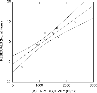
regression analysis. The scatter plot for these two variables (Fig.
15.8) suggests a
strong positive relationship. Just as we expected, the sites on the more productive
soils tend to have more hoes than expected, based on their size (positive residuals),
and those on the less productive soils tend to have fewer hoes than expected, based
on their size (negative residuals). The best-fit straight line looks to be quite a good
fit, and the 95% confidence zone around it is tight. The regression analysis fully
Table 15.3. Residual Numbers of Hoes and Soil
Productivity for Sites in the R´ıo Seco Valley
Residual Soil productivity
number of hoes (kg of maize per ha)
4.41 1,200
−1.68 950
1.14 1,200
−3.03 600
0.01 1,300
−1.38 900
−6.34 450
−0.93 1,000
−12.30 350
−3.67 750
4.55 1,500
10.00 2,300
6.93 1,650
2.30 1,700
216 CHAPTER 15
Figure 15.8. Scatter plot of residual number of hoes by soil productivity with best-fit straight line
and 95% confidence zone.
confirms all these observations. The correlation is very strong and highly significant
(r = 0.923, p < 0.0005). Since r
2
= 0.852, 85.2% of the variation in the residuals is
explained by soil productivity.
The results of these two regression analysis are complementary and contribute
cumulatively to our goal of explaining the variation in number of hoes at these sites.
The first regression analysis (number of hoes by site area) showed that site area
accounted for 53.5% of the variation in number of hoes, leaving 46.5% of the varia-
tion in number of hoes unexplained. It is that 46.5% of the variation left unexplained
by the first regression that is encapsulated in the residuals. The second regression
analysis (residual number of hoes by soil productivity) accounted for 85.2% of the
variation in hoe residuals, which was in turn the 46.5% of the variation in number of
hoes left unexplained by the first regression. This amounts, then, to 85.2% of 46.5%,
or 39.6% of the original variation in number of hoes. Together, the two regression
analyses explain 93.1% of the variation in number of hoes (53.5% in the first regres-
sion, and 39.6% in the second). Taken together, the two independent variables (site
area and soil productivity) explain quite a lot of the variation in number of hoes,
providing strong support for the interpretation that larger settlements had more craft
workers, elites, and others not engaged in farming, and that, in addition, settlements
located on more productive soils were more involved in farming. Not only are the
patterns of relationships between these variables strong, they are very highly signif-
icant, which tells us that our samples, small though they may be, are large enough
to give us great confidence that we are not just seeing the vagaries of sampling in
operation.
Just as the assessment of the proportion of variability explained is cumulative,
so are the equations for predicting the number of hoes at a site on the basis of the
two independent variables. We have already produced the regression equation for
RELATING A MEASUREMENT TO ANOTHER MEASUREMENT 217
predicting the number of hoes, based on the area of the site:
Number of hoes =(−1.959 ×Site area)+47.802
Now we can also predict the errors in that previous estimate (that is, the residuals):
Residual number of hoes =(.010 ×Soil productivity) −11.004
Since the residuals are the errors in the first prediction, adding the second equation
to the first produces a prediction of the number of hoes at a site that is based both
on its area and the productivity of the surrounding soils:
Number of hoes = {(−1.959 ×Site area)+47.802}
+{(.010 ×Soil productivity) −11.004}
There are, of course, residuals from the second regression analysis as well. If they
were large enough to be interested in, we could study their relationship with yet
another variable. In this way regression analysis allows for the combination of a
series of analyses of relationships between two variables, and produces an integrated
result of what has, in effect, become a multivariate analysis. Most statpacks will
perform multiple regression, which is an extension and elaboration of this basic idea.
ASSUMPTIONS AND ROBUST METHODS
It may come as a surprise that linear regression is not based on the assumption that
both measurements involved have normal shapes. The shape assumptions that we
must be alert to in linear regression have to do with the shapes of point distributions
in scatter plots. Just as we examine stem-and-leaf plots to check for the single peak
and symmetry that characterize a normal shape, we examine a scatter plot prior
to linear regression for the shape of point distributions. What we need to see is a
cloud of points of roughly oval shape. There should be no extreme outliers from the
cloud, the oval should be of similar thickness throughout, and there should be no
tendencies toward curvature of the whole oval. These three potential problems can
be discussed separately.
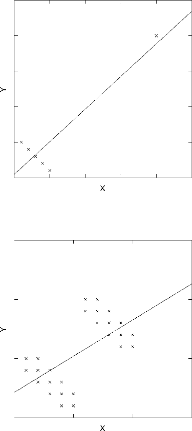
First, outliers present severe risks to linear regression. Fig.
15.9 provides an
extreme example that should make the principle intuitively clear. The points in
the lower left corner of the scatter plot clearly show an extremely strong negative
correlation. The single outlier to the upper right, however, will cause the best-fit
straight line to be as shown – a positive correlation of some strength. Outliers have
such a strong effect on the best-fit straight line that they simply cannot be over-
looked. When outliers are identified, those cases should be examined with great care
to see whether there is a measurement or data-recording error that can be corrected
or whether there is some other reason to justify excluding them from the sample.

218 CHAPTER 15
Statpacks
Regression analysis is hardly ever performed any more except by computer.
Different statpacks use a variety of vocabularies to talk about it, in part because
linear regression is only the tip of the iceberg. Regression analysis is really a
whole family of analytical approaches involving curved line fitting in addition
to straight line fitting and incorporating a number of variables simultaneously
instead of just two. Any very large and powerful statpack will perform many
of these other kinds of analysis as well, and the simple, but powerful, linear
regression techniques discussed here may be embedded in this broader family
of analyses. Consequently, the commands or menu selections that produce a
simple linear regression vary substantially from one statpack to another and
are often much more complicated than it seems like they need to be. Recourse
to the manual or help system for your particular program is likely to be nec-
essary. Some statpacks integrate scatter plots into the procedures that perform
regression analysis as an option, while others perform the numerical analysis
as one operation and produce scatter plots as a different operation. Usually the
inclusion of the curves delimiting a confidence region for the best-fit straight
line is an option to be specified as part of the production of a scatterplot. Resid-
uals, of course, are calculated as part of the regression analysis, but to be able
to use them as a new measurement and pursue further analysis with them it is
usually necessary to save them by specifying this as an option to the regression
analysis. Typically this results in the creation of a new data file in the normal
format your statpack uses for data files. The new file will have the same cases
as the original data file and a variable whose values are the residuals from the
regression analysis.
Second, oval shapes of points with very thin sections (or even worse, two or more
separate oval clouds) are the equivalent of multipeaked shapes for single batches
of numbers. They can create the same kinds of problems in linear regression that
outliers do. Fig.
15.10 shows another extreme example, where two ovals of points
showing negative correlations of some strength turn into a single best-fit straight line
with a positive slope when improperly analyzed together. Such a shape may occur
in a scatter plot of two variables that, when looked at individually, have clearly
single-peaked and symmetrical shapes. Shapes like this should be broken apart for
separate analysis.
Third, tendencies toward curved patterns in the oval of points can prevent a very
good fit of a straight line to a fundamentally linear pattern that just happens to
be curved. There are ways to extend the logic of linear regression to more com-
plex curvilinear relationships between variables, but it is usually much easier to
straighten out the curve by transforming one or both variables. The kinds of trans-
formations required are very like the transformations discussed in Chapter
5 and
may be applied to either or both of the variables to remove tendencies toward cur-
RELATING A MEASUREMENT TO ANOTHER MEASUREMENT 219
Figure 15.9. The devastating effect of a single outlier on the best-fit straight line.
Figure 15.10. The effect of two oval clouds of points on the best-fit straight line.
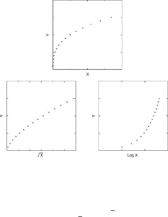
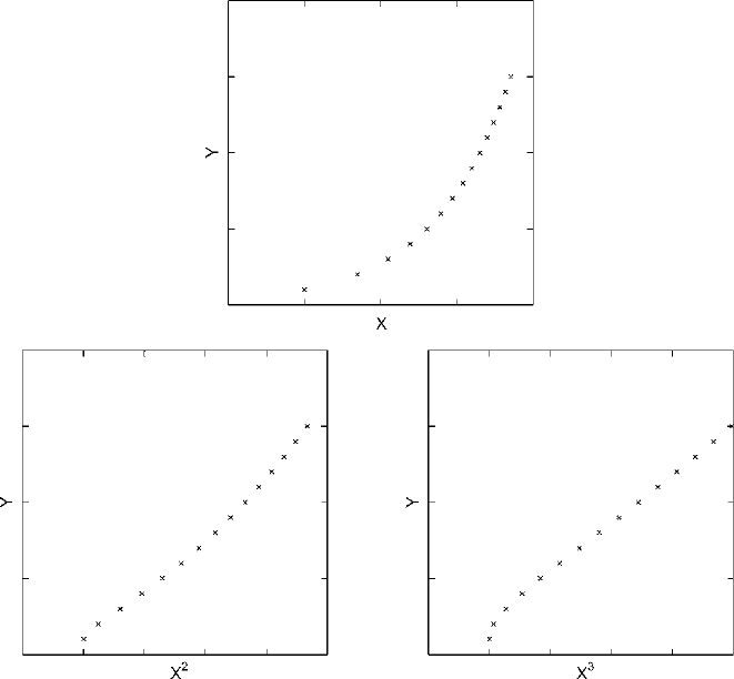
vature. As Fig. 15.11 illustrates, if the scatter plot shows a tendency toward linear
patterning but with the ends curving downward, a square root transformation of X
will produce a straighter line. If stronger corrective action is called for, the loga-
rithm of X can be used instead of the square root. Clearly, for the data in Fig.
15.11,
the logarithm of X is too strong a transformation, having produced just as curved
220 CHAPTER 15
Figure 15.11. The effect of transformations of X on a downward curvilinear pattern.
a pattern in the opposite direction. Fig. 15.12 illustrates transformations to correct
linear patterns where the ends curve upward. For these data the square of X pro-
duces good results. Using the cube of X produces a stronger effect than is needed
in this instance. Applying, for example, a square root transformation to X prior to
analysis means, of course, that it is not X but rather
√
X whose relationship to Y is
being investigated. Thus it becomes
√
X rather than X that is used in the regression
equation to predict the values of Y .
PRACTICE
You have excavated a site near Yenangyaung that has a number of apparent storage
pits containing artifacts and other debris. You wish to investigate whether the density
of artifacts (the number per unit volume) is constant for all the pits. (Another way
RELATING A MEASUREMENT TO ANOTHER MEASUREMENT 221
Figure 15.12. The effect of transformations of X on an upward curvilinear pattern.
to phrase this is to ask yourself whether, knowing the volume of a pit, you could
accurately predict the number of artifacts it contains.) The volume measurements
and the number of artifacts recovered from complete excavation of each pit are
given in Table
15.4.
1. Make a scatter plot of pit volume and number of artifacts. What does inspection
of the scatter plot suggest about a relationship between them?
2. Perform a regression analysis for pit volume and number of artifacts. How can
the relationship between number of artifacts and pit volume be expressed math-
ematically? How many artifacts would you expect to find in a pit whose volume
was 1.000m
3
?
3. How much of the variation in number of artifacts is “explained” by pit volume?
What is the statistical significance of the relationship between pit volume and

222 CHAPTER 15
Table 15.4. Data from Storage Pits at Yenangyaung
Vo l u m e ( m
3
) No. of Artifacts Volume (m
3
) No. of Artifacts
1.350 78 1.110 47
0.960 30 1.230 47
0.840 35 0.710 20
0.620 60 0.590 28
1.261 23 0.920 38
1.570 66 0.640 13
0.320 22 0.780 18
0.760 34 0.960 25
0.680 33 0.490 56
1.560 60 0.880 22
number of artifacts? Produce a scatter plot showing the 90% confidence region
for the best-fit straight line.
4. Sum up clearly and concisely what this regression analysis of the relationship
between pit volume and number of artifacts has shown.

Chapter 16
Relating Ranks
Calculating Spearman’s Rank Correlation ........................................................ 224
Significance ......................................................................................... 226
Assumptions and Robust Methods ................................................................ 228
Practice.............................................................................................. 228
Sometimes we have variables that at first glance appear to be measurements, but
that on further examination reveal themselves to be something less than actual mea-
surements along a scale. Often they really amount to relative rankings rather than
true measurements. For example, soil productivity is sometimes rated by producing
an index with an arbitrary formula using such values as content of various nutrients,
soil depth, capacity for water retention, and other variables that affect soil produc-
tivity. The formulas used in these ratings are carefully considered to produce a set
of numbers such that we are sure that higher numbers represent more productive
soils and lower numbers represent less productive soils. Such scales, for example,
would allow us to say that a rating of 8 means more productive soils than a rating
of 4. They seldom, however, leave us in position to say that a rating of 8 means soils
twice as productive as a rating of 4. It is our inability to make this last statement
that keeps such ratings from being true measurements. Instead, they are rankings.
Rankings allow us to put things in rank order (most productive soil, second most
productive soil, third most productive soil, etc.) but not to say how much more a
high ranking thing is than a low ranking thing.
The logic of linear regression relies on the measurement principle. (Think of the
scatter plots and the regression equations. If X is twice as large it places the corre-
sponding point twice as far over on the scatter plot. If X is twice as large it has twice
the effect on the prediction of Y by way of the regression equation.) If X is actually
only a ranking rather than a true measurement, then we should feel uncomfortable
about using regression. Instead of performing a linear regression and attempting
to predict the actual value of Y from X, we might use a rank order correlation
coefficient to assess the strength and significance of a rank order relationship.
A rank order relationship has nothing to do with the actual magnitude of the
rankings for either variable studied, but rather only with the order of the rankings. If
we rank order a batch of numbers according to the values for X and this rank order
is exactly the same as the rank order of values for Y,thenX and Y show a perfect
R.D. Drennan, Statistics for Archaeologists, Interdisciplinary Contributions
to Archaeology, DOI 10.1007/978-1-4419-0413-3
16,
c
Springer Science+Business Media, LLC 2004, 2009
223
224 CHAPTER 16
positive rank order relationship. That is, the highest value for X is for the case that
also has the highest value for Y ; the second highest value for X is for the case that
also has the second highest value for Y; and so on. A perfect negative rank order
relationship means that the case with the highest value for X has the lowest value
for Y; the case with the second highest value for X has the second lowest value for
Y; and so on until the case with the lowest value for X has the highest value for Y .
We can imagine a rank order correlation coefficient that works like Pearson’s r,
so that a perfect positive rank order relationship is assigned a value of 1; a perfect
negative rank order relationship is assigned a value of −1; and intermediate rela-
tionships are assigned values between 1 and −1, depending on the extent to which
the relationships approach one or the other of these ideal situations. Several such
coefficients exist. One of the most frequently used is Spearman’s rank correlation
coefficient (r
S
).
CALCULATING SPEARMAN’S RANK CORRELATION
Table 16.1 contains data for soil productivity ratings for 17 different soil zones in
the Konsankoro Plain. The Neolithic occupation consisted of a series of sedentary
village sites of remarkably consistent size. We take the number of village sites in
Table 16.1. Soil Productivity and Villages in the Konsankoro Plain
Soil Productivity No. of villages Rankings
zone rating per km
2
XYXYdd
2
t
x
T
x
t
y
T
y
A 2 0.26 3.52 1.52.25 2 0.5 1 0.0
B 6 1.35 11.514 −2.56.25 2 0.5 1 0.0
C 3 0.44 6 6 0.00.00 3 2.0 1 0.0
D 7 1.26 13.512 1.52.25 2 0.5 1 0.0
E 4 0.35 8.54 4.520.25 2 0.5 1 0.0
F 8 2.30 16 17 −1.01.00 3 2.0 1 0.0
G 8 1.76 16 16 0.00.00 3 2.0 1 0.0
H 1 0.31 1.53−1.52.25 2 0.5 1 0.0
I 3 0.37 6 5 1.01.00 3 2.0 1 0.0
J 5 0.78 10 11 −1.01.00 1 0.0 1 0.0
K 1 0.04 1.51 0.5 .25 2 0.5 1 0.0
L 8 1.62 16 15 1.01.00 3 2.0 1 0.0
M 7 1.34 13.513 0.5 .25 2 0.5 1 0.0
N 2 0.47 3.57−3.512.25 2 0.5 1 0.0
O 4 0.56 8.59−0.5 .25 2 0.5 1 0.0
P 3 0.48 6 8 −2.04.00 3 2.0 1 0.0
Q 6 0.76 11.510 1.52.25 2 0.5 1 0.0
∑
d
2
= 56.50
∑
T
x
=17.0
∑
T
y
= 0.0
