Drennan R.D. Statistics for Archaeologists: A Common Sense Approach

RELATING RANKS 225

each soil zone divided by the total number of square kilometers covered by that

zone to indicate how densely the zone was occupied, and we wish to investigate

whether more productive soil zones were more densely inhabited.

The ﬁrst step in calculating Spearman’s rank correlation is to determine the rank

orderings of all the cases for each of the two variables (taken separately). These rank

orderings are also given in Table 16.1. Ties frequently occur in the soil productivity

ratings. That is, for example, soil zones H and K are ranked in the lowest produc-

tivity category (1). These two least productive soil zones should be rank ordered 1

and 2, but we have no basis for putting one above the other since they are tied in

the productivity ratings. As a consequence, we assign each a rank order of 1.5 (the

mean of 1 and 2). Soil zones C, I, and P are tied with productivity ratings of 3. These

would be soil zones 5, 6, and 7 in rank order if we could determine which to put

above the other. Since we cannot make this determination, each is assigned a rank

order of 6 (the mean of 5, 6, and 7). Such a treatment is accorded whenever there are

ties. No ties occur in the number of villages per square kilometer (which actually is

a true measurement), so the rank ordering is simpler. It begins at 1 for soil zone K

and continues through zones A, H, and so on to zone F, which ranks 17th because it

has the highest number of village sites per square kilometer.

Subtracting the rank orderings for villages per square kilometer (Y) from the

rank orderings for soil productivity (X) gives us the difference between rankings d,

which we then square and sum up to get

∑

The last four columns in Table

16.1 concern a correction that must be made for

ties. The value t for each soil zone is the total number of soil zones that are tied at

that ranking. For example, soil zone A has a value of t

= 2 because a total of two

zones (A and N) are tied at its productivity rating of 2. Since there are no ties for

number of villages per square kilometer, all the values of t

are 1. For each t value

for each of the two variables, a value of T is obtained as follows:

T =

−t

The calculation of Spearman’s rank correlation requires three sums from

Table

16.1:

∑

,and

∑

. A sum of squares is calculated for each of the

two variables:

∑

−n

−

∑

where

∑

is from Table 16.1,andn is the number in the sample (17 in this

example). Thus, for the example in Table

16.1,

∑

−17

−17.0 = 408 −17 = 391 and

∑

−17

−0.0 = 408−0 = 408

Spearman’s rank correlation, then, is given by the equation

226 CHAPTER 16

Be Careful How You Say It

In conclusion to the example analysis in the text, we would say “There is a

strong and highly signiﬁcant rank-order correlation between soil productivity

and number of villages per square kilometer (r

= .93, p <.001).” This informs

the reader that the relationship is positive (more villages in more productive

soil zones), what correlation coefﬁcient was used, and just how unlikely it is

that the observed correlation would have occurred in this sample if there were

no correlation in the population from which the sample was selected.

∑

−

∑



∑

For the example in Table 16.1, then,

391 + 408 −56.5



(391)(408)

742.5

798.8

= 0.93

Spearman’s rank order correlation coefﬁcient, then, between soil productivity

and number of villages per square kilometer in the Konsankoro Plain is 0.93, indi-

cating a strong positive correlation. (Values for r

can be interpreted in much the

same manner as those for Pearson’s r, although the two cannot be compared directly.

That is, a Spearman’s r

of 0.85 between two variables cannot be said to indicate a

stronger correlation than a Pearson’s r of 0.80 between two other variables.)

If there are no ties, then we can easily see that

∑

T = 0 (as in the case of number

of villages per square kilometer in Table

16.1). If there are no ties for either variable,

then, there is no need to go to the trouble of ﬁguring t and T, and the entire equation

for Spearman’s rank correlation is considerably simpliﬁed:

= 1 −

∑

−n

SIGNIFICANCE

As usual, the question of signiﬁcance is “How likely is it that the correlation

observed in the sample is not a consequence of a correlation in the population that

the sample was selected from but instead simply a result of the vagaries of sam-

pling?” Put another way, “How likely is it that a sample this size with a correlation

this strong could be selected from a population where there is no correlation?” For

samples of ten or more, this question can be answered with the familiar t table

RELATING RANKS 227

Statpacks

Spearman’s rank correlation coefﬁcient is only one of several similar

approaches to evaluating the strength and signiﬁcance of rank order corre-

lations. Many statpacks provide options for calculating them all under the

heading of rank correlations or nonparametric correlations. Sometimes, r

calculated as an option with the same commands that produce Pearson’s r.

Even if your statpack does not provide Spearman’s rank correlation as a spe-

ciﬁc option, you still may be able to trick it into producing r

. It turns out

that Spearman’s rank correlation is equivalent to Pearson’s r calculated on

rankings. Consequently, you can provide rankings for each of your cases on

the variables you are interested in (the fourth and ﬁfth columns in Table

16.1)

and use your statpack to perform a regression analysis on those variables. The

resulting correlation coefﬁcient will be equivalent to r

(Table 9.1). The following formula gives the value of t:

t = r



n −2

1 −r

In our example,

t = .93



17 −2

1 −0.93

= 0.93



1 −0.86

= 0.93

√

107.14 = 9.63

Looking this value up in Table

9.1,usingtherowforn–1= 16 degrees of free-

dom, we discover that this value of t would be far beyond the rightmost column in

the table. The associated probability, then, would be far less than 0.001. Thus there

is far less than one chance in 1,000 that a sample of 17 would show a Spearman’s

rank correlation this strong if it had been selected from a population where there

was no rank order relationship between the two variables.

It should be noted that this example raises some complicated questions of what

population the data are a sample from. The sample consists of 17 soil zones that have

been surveyed. In order to accomplish the analysis we have just done, we must take

these 17 soil zones as a random sample from a larger and vaguely deﬁned population

of soil zones that are or might be in the Konsankoro Plain. This sample has given us

what we take to be 17 separate and independent observations for the two variables,

and these 17 observations form the batch that we have analyzed as a sample. Strictly

speaking, this is not a random sample from a population of soil zones. Indeed, this

sample may represent a complete survey of the entire Konsankoro Plain. If we have

studied the entire population, it may seem to make little sense to treat the data as

a sample. In evaluating signiﬁcance, however, we frequently engage in a sort of

228 CHAPTER 16

Table 16.2. Probability Values for Spearman’s Rank Correlation r

for Samples of Less Than 10

Conﬁdence 80% 90% 95% 99%

.80 .90 .95 .99

Signiﬁcance 20% 10% 5% 1%

.20 .10 .05 .01

4 .639 .907 1.000

5 .550 .734 .900 1.000

6 .449 .638 .829 .943

7 .390 .570 .714 .893

8 .352 .516 .643 .833

9 .324 .477 .600 .783

(Adapted from “Distributions of Sums of Squares of Rank Differences for Small Numbers of

Individuals” by E.G. Olds (Annals of Mathematical Statistics 9:133–148 [1938])

pretend sampling from an imaginary larger population. What we learn from the

evaluation of signiﬁcance in a case like this is still, however, whether we should

have much conﬁdence in the correlation observed. What we have found out in this

instance is that the correlation we observed is not at all likely to be pure random

chance at work in a small sample. We will consider this notion of pretend sampling

further in Chapter 20.

The formula for values of t is appropriate only if the sample is ten or more. If the

size of the sample is less than ten, then Table

16.2 should be used to determine the

associated probability.

ASSUMPTIONS AND ROBUST METHODS

Since Spearman’s rank correlation does not assume normal distributions, or rely on

means, standard deviations, or scatter plots, it is automatically highly robust. No

transformations or other modiﬁcations need ever be applied. This, in effect, makes

a very robust correlation coefﬁcient that can be used instead of Pearson’s r when

such factors present problems for the application of Pearson’s r.

PRACTICE

You have excavated the remains of 12 dwellings in the village site of Teixeira. You

notice that some of the artifacts recovered from the dwelling areas are ﬁner and

RELATING RANKS 229

Table 16.3. Floor Area and Artifact Status Index for

12 Excavated Houses from the Teixeira Site

Status index Floor area (m

)

23.4 31.2

15.8 28.6

18.3 27.3

12.2 22.0

29.9 45.3

27.4 33.2

24.2 30.5

15.6 26.4

20.1 29.5

12.2 23.1

18.5 26.4

17.0 23.7

fancier than others, and might indicate differences in status or wealth between the

households. You identify a variety of ornamental objects and pottery with incised

decoration as possible status indicators, and you count the number of such artifacts

in each household area per 100 artifacts recovered. This gives you an index of status

or wealth based on the artifact assemblages in the different households. You wish to

investigate whether this status index is related to the size of the dwelling structure

itself (pursuing the idea that wealthier families might have larger houses). The data

are given in Table

16.3

1. How strong and how signiﬁcant is the relationship between house ﬂoor area and

your status index?

2. What sort of support do your observations provide for the idea that wealthier

households (as indicated by their possessions) had larger houses?

Chapter 17

Sampling a Population with Subgroups

Pooling Estimates .................................................................................. 234

The Beneﬁts of Stratiﬁed Sampling ............................................................... 236

When the population we are interested in has subgroups that we are also interested

in separately, it is often useful to select a separate sample of elements from each of

the subgroups. For such purposes each subgroup is treated as if it were a completely

separate population. A sample of whatever size is needed is selected from each of

these separate populations, and the values of interest are estimated separately for

each population. Suppose that we have reliable information on the locations of all

sites in a region. No one has attempted to discover the sizes of these sites, however.

We could select a sample of the known sites and go make systematic surface collec-

tions in an effort to determine how large they are. These determinations could then

form the basis for estimating the mean site size for the region. If, in addition, the

region could be divided into three different environmental settings (remnant levees,

river bottoms, and slopes) we might be interested in estimating the mean site area

for each of the settings.

Table

17.1 provides information on a sample of sites for each of these three set-

tings, as well as a stem-and-leaf plot for each sample. The table gives N, the total

number of sites in each setting (the three populations sampled), and n, the number

of sites in each of the three samples. The stem-and-leaf plots show a single-peaked

and symmetrical shape for each of the samples, and their standard errors have been

calculated using the ﬁnite population corrector (Chapter

9) since the sampling frac-

tions are large. Multiplying these standard errors by the corresponding values of t

for 95% conﬁdence and n −1 degrees of freedom gives us error ranges to attach to

the estimated mean site areas for each of the three settings. Thus we are 95% con-

ﬁdent that the mean area of sites on remnant levees is 1.71ha±0.32ha; in the river

bottoms, 2.78ha±0.31ha; and on the slopes, 0.83ha±0.32 ha.

R.D. Drennan, Statistics for Archaeologists, Interdisciplinary Contributions

to Archaeology, DOI 10.1007/978-1-4419-0413-3

17,

 Springer Science+Business Media, LLC 2004, 2009

233

234 CHAPTER 17

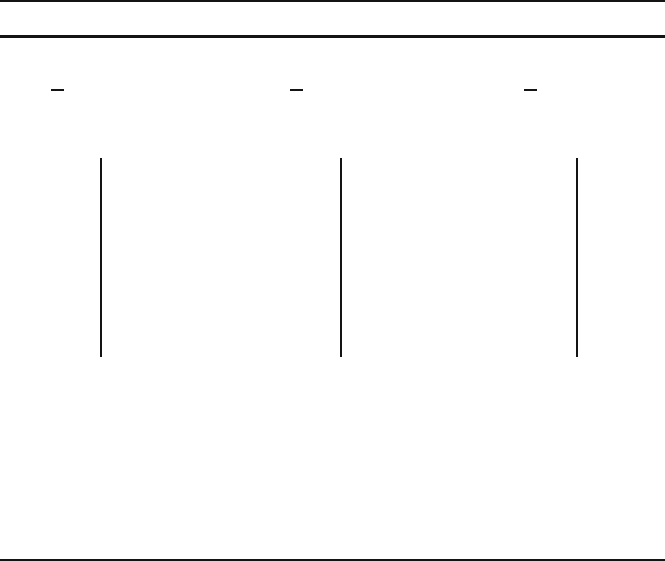
Table 17.1. Site Areas (ha) in Three Settings

River Bottoms Remnant Levees Slopes

N = 53 N = 76 N = 21

n = 12 n = 19 n = 7

X = 2.78 X = 1.71 X = 0.83

SE = 0.14 SE = 0.15 SE = 0.13

3.3 2.9 0.7

2.7 4

1.7 4 1.3 4

2.1 3 81.33 1.2 3

3.8 3 134 2.1 3 20.63

2.7 2 7789 1.9 2 59 0.6 2

3.4 2 144 1.2 2 0113 1.2 2

2.9 1 82.5166779 0.2 1

2.8 1 2.1 1 0234 1 223

2.4 0

1.6 0 78 0 667

1.8 0

1.7 0 402

2.4 2.0

3.1 1.6

1.0

1.4

2.3

3.2

0.8

0.4

0.7

These estimates and their 95% conﬁdence error ranges conﬁrm what we might

well have suspected from looking at the three stem-and-leaf plots – sites in the three

settings have markedly different mean sizes, and the differences that we observe

between our three samples are not at all likely to be just the result of sampling

vagaries. Up to this point, we have done nothing more than treat these three samples

in the ways discussed in Chapter

POOLING ESTIMATES

At this point, however, we might well want to consider the three samples together

in order to talk about sites in the region in general, irrespective of the settings in

which they were located. We cannot simply put all the sites from all three samples

together into one sample, though, and consider it a random sample of sites in the

region. Such a sample would most deﬁnitely not be a random sample of the sites in

the region because the selection procedures did not give each site in the region an

equal chance of selection. Of the 21 sites on the slopes, 7 (or 33.3%) were selected;

SAMPLING A POPULATION WITH SUBGROUPS 235

of the 53 sites in the river bottoms, 12 (or 22.6%) were selected; and of the 76

sites on remnant levees, 19 (or 25.0%) were selected. Thus river bottom sites had

less chance of being included in the sample (a probability of 0.226) than sites on

levees (a probability of 0.250), and levee sites had less chance of being included

than sites on the slopes (a probability of 0.333). The overall sample produced by just

putting these three separate samples together would systematically over-represent

slope sites and systematically under-represent river bottom sites. Any conclusions

we might arrive at about mean site area in the region as a whole based on such a

sample would be affected by these sampling biases.

What we must do is consider the larger problem one of stratiﬁed sampling,

as selecting separate samples from different subgroups of a population is usually

called. In this example, each of the three environmental settings would be a sampling

stratum. Each sampling stratum would form a population to be sampled separately

from the other sampling strata, just as we have done in this example. Appropriate

sample sizes and sampling procedures would be determined independently for each

sampling stratum, and the samples selected would be used independently to make

estimates about each of the parent populations. We have already done all of this. It

raises no new issues in sampling beyond those dealt with in Chapters

7–11.

Only at the last step, that of pooling the estimates made for each sampling stratum

into an overall estimate for the whole population must special steps be taken. In

the ﬁrst place, having already discovered that sites in the three different settings

have rather different mean areas, we must consider whether it makes any sense

even to speak of the mean area of sites for the region as a whole. If the overall

population of sites had a shape with multiple peaks, it would be foolish to attempt

any analysis of the entire set of sites as a single batch. We do not, of course, have any

way of knowing for certain what the shape of the whole population would be, but,

since the sampling fractions in the three sampling strata are not wildly different, we

could look at a stem-and-leaf plot of all three samples together to get a rough idea.

Such a stem-and-leaf plot appears in Table

17.2. It is certainly single peaked and

symmetrical enough to make it meaningful to use the mean as an index of center

for the whole batch. Thus, we could consider it sensible to make an estimate of

Table 17.2. Stem-and-Leaf Plot

of Areas of Sites from

All Three Samples in Table

17.1

3 8

1234

577899

0111344

667789

0222334

66778

236 CHAPTER 17

the mean site area for all sites in the region by pooling the estimates for the three

sampling strata, as follows:

∑





where

= the pooled estimate of the mean, that is, the estimated mean for the

entire population, taking all sampling strata together,

= the mean of the elements

in the sample for stratum h, N

= the total number of elements in the population of

stratum h,andN = the total number of elements in the entire population.

For the example from Table

17.1,

(76)(1.71)+(53)(2.78)+(21)(.83)

150

294.73

150

= 1.96ha

Thus we estimate that the mean area of sites in the region as a whole (irrespective

of environmental setting) is 1.96 ha. We attach an error range to this estimate in

a similar fashion, by pooling the standard errors for the three separately selected

samples:



∑







where SE

= the pooled standard error for all sampling strata taken together, SE

the standard error for sampling stratum h, N

= the total number of elements in the

population of stratum h (as before), and N = the total number of elements in the

entire population (also as before).

For the example from Table

17.1,



(76

)(.15

)+(53

)(.14

)+(21

)(.13

)

150

13.87

150

= .09

This pooled standard error is treated like any other. To produce an error range for

95% conﬁdence, we would multiply it by the value of t corresponding to 95% conﬁ-

dence and n−1 degrees of freedom where n is now the number in all three samples

considered together, or 38. This value of t is 2.021, so we would be 95% conﬁdent

that the mean area of all sites in the region is 1.96ha±0.18 ha.

THE BENEFITS OF STRATIFIED SAMPLING

Stratiﬁed sampling can sometimes offer a more precise estimate for an entire pop-

ulation than simply sampling the entire population directly. This makes stratiﬁed

sampling potentially useful even in situations where we might not be much inter-

ested in the separate means of the sampling strata. The possible increased precision

comes from providing a smaller error range in the situation where a population

has subgroups whose means differ somewhat from each other but which have very

SAMPLING A POPULATION WITH SUBGROUPS 237

small standard deviations when each is taken separately. That is, if the subgroups

each form batches with smaller spreads than the population as a whole, the error

ranges associated with the estimates of their means may be quite small. When these

are pooled into an error range for the estimated overall population mean it may well

be smaller than the error range that would have been obtained from a single sample

drawn randomly from the population as a whole. Sometimes this effect is strong

enough to outweigh the opposite effect resulting from the fact that the samples from

the subgroups are each smaller than the total sample. If a population is easily divided

into subgroups whose means may be different and whose members vary little from

each other, then it is worth considering sampling that population by those subgroups

instead of as a whole, even if the subgroups are of little intrinsic interest separately.

Drennan R.D. Statistics for Archaeologists: A Common Sense Approach

Подождите немного. Документ загружается.