Drennan R.D. Statistics for Archaeologists: A Common Sense Approach

Подождите немного. Документ загружается.

194 CHAPTER 14

Table 14.7. Regional Survey in Three Environmental Settings

No. of

sites

%oftotal

sites

Area surveyed

Environmental setting km

%oftotal

Remnant levees 19 50.03.928.7

River bottoms 12 31.68.361.0

Slopes 7 18.41.410.3

Totals 38 100.013.6 100.0

Table 14.8. An Incorrect Way to Tabulate Observed Values

from Table 13.7 for a Chi-Square Test

No. of sites Area surveyed (km

)

Remnant levees 19 3.9

River bottoms 12 8.3

Slopes 7 1.4

In this example, what we have is a sample of 38 sites. If we are willing to treat

this as a random sample of sites in the region, then we can compare the propor-

tions of sites in different settings to the theoretical expectation based on how the

territory surveyed to ﬁnd the 38 sites was divided between the three different set-

tings. One way to do this would be to follow the approach discussed in Chapter

for estimating the proportions of sites in different settings and for attaching error

ranges to these estimates. This would tell us, for instance, that we can have 99%

conﬁdence that our sample of 38 sites came from a population in which 31.6% ±

20.3% of the sites were located in the river bottoms. (You can calculate this yourself,

following the procedure in Chapter

11.) If prehistoric inhabitants showed no pref-

erence for any of these environmental settings, however, the proportion we would

have expected here was 61.0%, since 61.0% of the territory is in this zone. This

proportion is considerably higher than the top of the 99% conﬁdence error range

(51.9%), and so we can say that it is extremely unlikely that our sample came from

a population with 61.0% sites in the river bottoms. Although we do ﬁnd sites there,

it seems that the prehistoric inhabitants showed something of an aversion to settling

in the river bottoms. (Or possibly that recent sedimentation has covered more sites

in the river bottoms than elsewhere, resulting in a particular failure to discover such

sites on survey. This is a question of interpretation that statistical analysis of these

numbers will not help us with.)

If we want to know exactly how unlikely it is that our sample came from a pop-

ulation with 61.0% sites in the river bottoms, we could perform a one-sample t test,

as discussed in Chapter

12. This example is different from the example one-sample

t test in Chapter

12 only in that there are three categories involved rather than just

two. We could follow this approach to each of the three categories, determining

COMPARING PROPORTIONS OF DIFFERENT SAMPLES 195

whether the proportion estimated on the basis of our sample was greater or less

than we would expect and how likely it was that the difference observed could be

attributed to the amount of random variation ordinarily seen in samples the size of

ours. This would lead to a speciﬁc discussion of settlement preferences (or apparent

lack thereof) in regard to each of the three environmental settings.

We might want to treat the issue in a more comprehensive way, however, focusing

not on each individual category, but asking the more general question, “How likely

is it that this entire sample of 38 sites came from a population of sites in which there

was no preference for locating sites in any particular environmental setting?” We

can use a chi-square test to answer this question, but not in the way indicated in

Table

14.8. Instead, we use the information we have to determine expected numbers

of sites in each environmental setting as in Table

14.9. Since 28.7% of the surveyed

area was on remnant levees, we might expect 28.7% of the 38 sites found (10.9

sites) to be on remnant levees, and so on. We now have a one-variable tabulation –

observed and expected values for three categories. We can use these observed and

expected values to calculate

just as before:

∑

−E

)

(19 −10.9)

10.9

(12 −23.2)

23.2

(7 −3.9)

3.9

= 6.0192 + 5.4069 + 2.4641

= 13.8902

Since there is only one row in this table (or one column – it makes no difference

whether the table is vertical or horizontal), the number of degrees of freedom is

one less than the number of categories. Here, there are three categories, so two

degrees of freedom. A value of 13.8902 for

is just beyond the rightmost column

of Table

14.4 in the row for two degrees of freedom. The rightmost column is for sig-

niﬁcance of .001. We could thus conclude, “It is extremely unlikely that this sample

of sites was selected from a population in which sites were evenly distributed across

environmental settings (

= 13.8902, p <.001).” Or, “The difference between our

survey results and the expected results was very highly signiﬁcant (

= 13.8902,

p <.001).”

Table 14.9. Observed and Expected Numbers of Sites

for Chi-Square Test

No. of sites

Area surveyed Exp. Obs.

Remnant levees 28.7% 10.9 19

River bottoms 61.0% 23.2 12

Slopes 10.3% 3.9 7

Totals 100.0% 38 38

196 CHAPTER 14

PRACTICE

1. You have made surface collections at the Granger and Rawlins sites. Both col-

lections include the same kinds of pottery, and you want to investigate whether

the two sites differ in regard to the proportions of different pottery types. At the

Granger site, you collected 162 sherds of the type Serengeti Plain, 49 sherds of

the type Mandarin Orange, and 57 sherds of the type Zane Gray; from the Rawl-

ins site you have 40 sherds of Serengeti Plain, 43 sherds of Mandarin Orange, and

49 sherds of Zane Gray. After considering possible sampling biases, you decide

to use the collections as random samples from the populations consisting of all

the sherds in each site. Estimate the proportions of the three pottery types at each

site. Draw a bullet graph comparing the estimated proportions for the two sites

with error bars for the 80%, 95%, and 99% conﬁdence levels. (Think carefully

about how to arrange the graph so that the error ranges you want to compare to

each other are most easily compared.) How conﬁdent are you that the two sites

differ in regard to proportions of ceramic types? Summarize the conclusions of

your graphical comparison in one or two sentences.

2. Approach the issues raised in Question 1 by evaluating the strength and signiﬁ-

cance of the association between the variables site and pottery type. Summarize

your results in one sentence. How do these results compare with those obtained

in Question 1? What are the advantages and disadvantages of approaching these

issues with a chi-square test rather than by estimating population proportions?

Table 14.10. Temper and Surface Finish for Sherds from the Opelousas Site

Temper Surface Temper Surface Temper Surface

Sand Red Shell Plain Shell Red

Sand Red Sand Plain Shell Red

Sand Red Shell Red Sand Plain

Shell Plain Shell Plain Sand Plain

Sand Red Sand Red Sand Red

Sand Plain Shell Plain Sand Red

Sand Red Shell Red Sand Plain

Shell Plain Sand Red Sand Red

Shell Red Shell Red Shell Plain

Shell Red Shell Red Sand Red

Sand Plain Sand Plain Sand Red

sand Red Sand Red Sand Red

Sand Red Shell Plain Shell Red

Sand Plain Shell Red Shell Plain

Sand Plain Sand Red Shell Red

Shell Plain Sand Plain Shell Plain

Shell Plain Sand Plain

Shell Red Shell Plain

COMPARING PROPORTIONS OF DIFFERENT SAMPLES 197

3. From the Opelousas site you have recovered a pitifully small collection of eroded

sherds. You can’t tell much about them except that some are tempered with shell

and some with sand and that some were ﬁnished with a red slip while others

have plain surfaces. The complete data are given in Table

14.10. Investigate the

statistical signiﬁcance and strength of any association between temper material

and surface ﬁnish with the sample that you have. Summarize the meaning of your

results in one clearly worded sentence.

Chapter 15

Relating a Measurement Variable to Another

Measurement Variable

Looking at the Broad Picture ...................................................................... 200

Linear Relationships................................................................................ 201

The Best-Fit Straight Line ......................................................................... 204

Prediction ........................................................................................... 207

How Good Is the Best Fit? ......................................................................... 209

Signiﬁcance and Conﬁdence ....................................................................... 211

Analysis of Residuals .............................................................................. 213

Assumptions and Robust Methods ................................................................ 217

Practice.............................................................................................. 220

In Chapters 12 and 13 we investigated the relationship between a measurement vari-

able and a categorical variable. We took two approaches to this task. The ﬁrst was

to estimate population means for the measurement variable in each of the cate-

gories of the categorical variable and attach error ranges to those estimates. The

second approach was to use either a two-sample t test (if only two categories were

involved) or an analysis of variance (if more than two categories were involved). In

Chapter

14 we investigated the relationship between two categorical variables. Once

again we took two approaches. The ﬁrst was to estimate population proportions for

one of the variables in each of the categories of the other variable and attach error

ranges to those estimates. The second approach was to use a chi-square test to eval-

uate signiﬁcance and Cramer’s V to evaluate strength of association. There remains

only to investigate the relationship between two measurement variables to complete

all the possible combinations, and that is the subject of this chapter. We will see

that one approach here is so powerful that we will not really consider alternative

approaches.

Table

15.1 provides an example set of data consisting of observations on 14

known sites of the Oasis phase in the R´ıo Seco valley. At each of the sites a system-

atic program of surface collection was undertaken to produce a sample of exactly

100 artifacts. After careful consideration of sources of bias we decide that we are

willing to work with this sample of sites as if it were a random sample. Similarly

considering sources of bias for the artifact collections, we decide we are willing

to treat each as if it were a random sample of artifacts on the surface. Since each

collection consists of 100 artifacts, the number of hoes in each is the percentage of

hoes in the collection, and simultaneously our best approximation of the percentage

R.D. Drennan, Statistics for Archaeologists, Interdisciplinary Contributions

to Archaeology, DOI 10.1007/978-1-4419-0413-3

15,

 Springer Science+Business Media, LLC 2004, 2009

199

200 CHAPTER 15

Table 15.1. Observations of Site Area and Number of Hoes in Collections of 100

Artifacts Made at Oasis Phase Sites in the R´ıo Seco Valley

Site area Number of hoes Site area Number of hoes

(ha) Per 100 artifacts (ha) Per 100 artifacts

19.0 15 12.7 22

16.4 14 12.0 12

15.8 18 11.3 22

15.2 15 10.9 31

14.2 20 9.6 39

14.0 19 16.2 23

13.0 16 7.2 36

of hoes in each population (that is, the population of artifacts on the surface at each

of the sites). In effect, of course, what we are dealing with here is a percentage, and

percentages like this make perfectly suitable measurement variables to study in this

way. What we want to investigate here is whether there is any relationship between

the area of the site, as indicated by the extent of artifacts visible on the surface, and

the number of hoes collected in the 100-artifact sample.

LOOKING AT THE BROAD PICTURE

As usual, drawing a plot that presents a picture of important aspects of the patterns

to be observed is a good way to begin. The relationship between two measurement

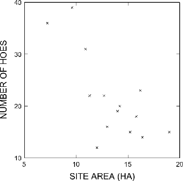
variables is best illustrated by a scatter plot (Fig.

15.1). Each x in the scatter plot

represents one of the sites, and its position is determined according to the area of

the site (in the horizontal direction) and the number of hoes in the collection of 100

artifacts (in the vertical direction).

Simple observation of this scatter plot begins to reveal something of the relation-

ship between these two variables. The points toward the left of the graph (that is,

with low values for site area) tend to fall fairly high on the graph (that is, they have

high values for number of hoes). The points farther toward the right of the graph

(that is, with high values for site area) tend to fall fairly low on the graph (that is

they have low values for hoes). This suggests a pattern of larger sites having rela-

tively fewer hoes per 100 artifacts and smaller sites having relatively more hoes per

100 artifacts.

In looking for patterns in scatter plots, especially if they are not very clear, it may

sometimes help to look at groups of points separately and think of the levels in these

sub-batches. For example, look at the points representing small sites (between 5 and

10 ha) in Fig.

15.1. There are only two such small sites, and both points fall very

high on the graph, indicating that both sites have very high numbers of hoes. The

center of this small batch of two sites is clearly quite high, perhaps around 37 hoes.

In fact, these two smallest sites have the largest numbers of hoes of all the sites.

RELATING A MEASUREMENT TO ANOTHER MEASUREMENT 201

Figure 15.1. Scatter plot of number of hoes per 100 artifacts collected by site area.

Next look at the points in Fig. 15.1 that represent the middle-sized sites (between 10

and 15 ha). All these points fall lower on the graph than the points representing the

small sites. The center of this batch of middle-sized sites falls lower than the center

for the small sites, probably somewhere near 20 hoes. Clearly the middle-sized sites

have fewer hoes than the small sites. Finally, look at the points representing the

large sites (between 15 and 20 ha). The center of this batch is lower still, perhaps

around 15 hoes. The same pattern emerges from this more detailed examination of

the scatter plot that we saw on simple inspection: in general, the bigger the site, the

smaller the number of hoes per 100 artifacts.

This detailed way of looking at the scatter plot suggests one way we could

approach this problem. We could treat site area as three categories (small, medium,

and large) and estimate the mean number of hoes per 100 artifacts in each of these

categories. Then we could attach error ranges to these estimates and draw a bullet

graph to illustrate the overall patterns. Or we could perform an analysis of variance

– the other technique applicable to investigating the relationship between a measure-

ment and a set of categories. Measurement variables can always be converted into a

set of categories in this way, and sometimes it is useful to do so. There is, however, a

much more powerful way to approach the investigation of the relationship between

two measurements.

LINEAR RELATIONSHIPS

The easiest kind of relationship to describe between two measurements is a linear,

or straight-line, relationship. Such a relationship is called linear because it is repre-

sented by a straight line on a scatter plot. Perhaps the simplest possible relationship

between two measurements is when the one equals the other. If we let X represent

202 CHAPTER 15

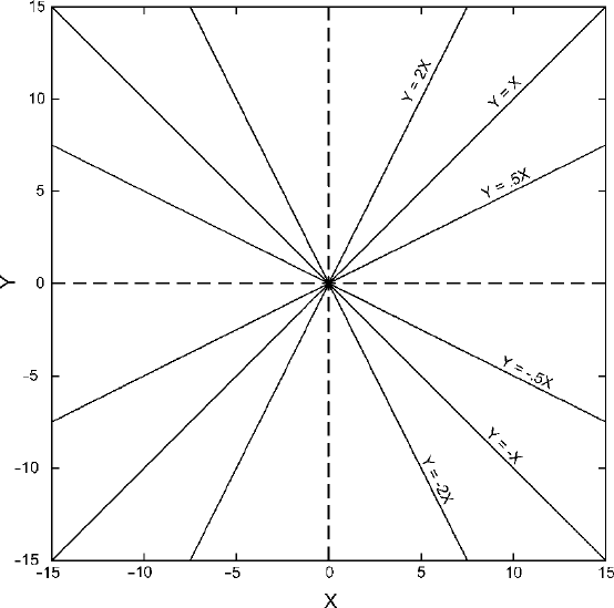
Figure 15.2. Some plotted straight lines and the equations that correspond to them.

one of the measurements and Y represent the other, then the relationship of equiva-

lence is simply expressed by the equation Y = X. For any given value of X,thereisa

corresponding value of Y, which is determined easily by the equation. For example,

when X = 5, then Y = 5; when X = −10, then Y = −10. The values of X and Y

are plotted on the graph in Fig.

15.2. (By convention we always use the horizontal

axis for X and the vertical axis for Y.) All the points representing pairs of X and Y

values that satisfy the equation Y = X, lie along the line labeled Y = X in Fig.

15.2

– a perfect straight-line relationship between X and Y .

The other lines in Fig.

15.2 also represent perfect straight-line relationships

between X and Y. They are labeled with the corresponding equations. The positions

of these lines can be determined experimentally. For example, the line that repre-

sents Y = −2X is deﬁned by all the points that satisfy the equation Y = −2X.These

include X = 5, Y = −10; X = −7, Y = 14 and so on. The equations in Fig.

15.2 are

algebraic expressions of relationships between two measurements and the lines on

the graph are geometric expressions of the same relationships. Each equation com-

prises a complete description of the corresponding line. If this is at all unclear, it is a

good idea to experiment on your own with some equations and their corresponding

RELATING A MEASUREMENT TO ANOTHER MEASUREMENT 203

Figure 15.3. More plotted straight lines and the equations that correspond to them.

graphs. Make up some values for X; calculate the corresponding values for Y;and

plot the points.

Comparison of the equations in Fig.

15.2 reveals one property of the relationship

between equations and lines. If Y simply equals X multiplied by some number, then

the relationship is represented geometrically by a straight line, and that straight line

passes through the origin of the graph. (The origin is the point where X = 0and

Y = 0.) The number by which X is multiplied in the equation is called the coefﬁcient

of X, and it is this coefﬁcient that governs the slope of the line. If the coefﬁcient of

X is positive, then the line rises as it moves from left to right. If the coefﬁcient is

negative, then the line falls as it moves from left to right. The larger the absolute

value of the coefﬁcient, the steeper the slope. That is, Y = 2X has a steeper slope

than Y = .5X;andY = −2X has a steeper slope than Y = −.5X. (In the equation

Y = X, of course, the coefﬁcient of X is 1.)

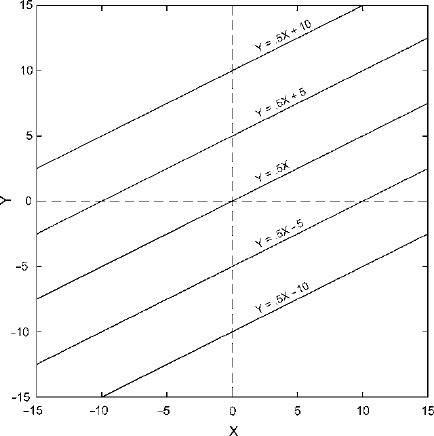
Figure

15.3 illustrates the other principal characteristic of straight lines on a

graph – their positions relative to the origin. All the lines on the graph in Fig.

15.3

have the same slope – the coefﬁcient of X is .5 in every case. They differ, however,

in the degree to which they are offset from the origin. These equations differ only

in having an additional term added to the product of X and its coefﬁcient. The line

corresponding to Y = .5X + 5 crosses the Y axis at the point where Y = 5. (This, of

course, has to be true because X is 0 at the Y axis, and when X = 0thenY = 5.)

This additional term is called the Y intercept since it is the value of Y when X is 0,

whichistosay,thevalueofY where the straight line crosses the Y axis.

204 CHAPTER 15

Thus for any straight-line relationship between X and Y we can write an equation

in the form

Y = bX + a

where b = the slope of the line, and a = the Y intercept, or value of Y where the line

crosses the Y axis.

This speciﬁes exactly what the relationship between X and Y is. It enables us to

say, for a given value of X,whatY will be. By convention, we always take X as a

given, and let Y’s value depend on X. Thus X is the independent variable and Y is

the dependent variable.

THE BEST-FIT STRAIGHT LINE

We have strayed rather far from the example where we wanted to investigate the

relationship between site area and number of hoes collected per 100 artifacts. The

point of the discussion of straight-line relationships, however, was to make clear

exactly what kind of mathematical relationship we might expect to ﬁnd between

these two measurements. If the relationship between site area and number of hoes

collected can be described reasonably accurately as a straight-line relationship, then

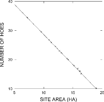
we can characterize it in these terms. If, for example, the scatter plot in Fig.

15.1 had

looked like Fig.

15.4 instead, we would ﬁnd it quite easy to apply the principles of

straight-line equations just discussed. The points in Fig.

15.4 do fall almost perfectly

along a straight line, and an approximation of that line has been drawn on the graph.

We could measure the slope of the line and determine the Y value of the point at

Figure 15.4. If the scatter plot in Fig. 15.1 had looked like this, it would have been easy to ﬁt a

straight line to the points.