Drennan R.D. Statistics for Archaeologists: A Common Sense Approach

Подождите немного. Документ загружается.

RELATING A MEASUREMENT TO ANOTHER MEASUREMENT 205

which it crosses the Y axis and write an equation that speciﬁed the relationship

between the two measurements algebraically.

The problem, of course, is that the points in the real scatter plot from our example

data did not fall almost perfectly along a straight line. While the general pattern of

declining numbers of hoes per 100 artifacts with increasing site area was clear, no

straight line could be drawn through all the points. There are so many advantages

to working with straight-line relationships, though, that it is worth trying to draw a

straight line on Fig.

15.1 that represents the general trend of the points as accurately

as possible – a best-ﬁt straight line. The statistical technique for accomplishing this

is linear regression.

The conceptual starting point for linear regression is to think exactly what cri-

terion would determine which line, of all the possible straight lines we could draw

on the scatter plot, would ﬁt the points best. Clearly, we would like as many of the

points as possible to lie as close to the line as possible. Since we take the values of

X as given, we think of closeness to the line in terms of Y values only. That is, for a

given X value, we think of how badly the point “misses” the line in the Y direction

on the graph. These distances are called residuals, for reasons that will become clear

later on.

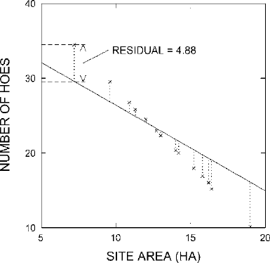
We can explore the issue of residuals with the completely ﬁctitious scatter plot

of Fig.

15.4. Since the points in this scatter plot do fall very closely along a straight

line, it is a bit easier to see good and bad ﬁts. Fig.

15.5 illustrates a straight line

that does not ﬁt the pattern of points nearly so well as the one in Fig.

15.4. We can

see that simply by inspection. We could put a ﬁner point on just how bad the ﬁt is

by measuring the residuals, which are indicated with dotted lines in Fig.

15.5.The

measurements, of course, would be taken vertically on the graph (that is, in the Y

Figure 15.5. A straight line that does not ﬁt the points from Fig. 15.4 very well.

206 CHAPTER 15

direction) and would be in terms of Y units (that is, in this example, in terms of

numbers of hoes). The same operation could be performed algebraically as well.

Since the line corresponds to a speciﬁc linear equation relating X and Y, we could

use that equation to calculate, for each X value, the value of Y that would be “cor-

rect” according to the relationship the line represents. The difference between that

“correct” value of Y and the actual value of Y would correspond to the graphical

measurement of the residual. The residual and its measurement are shown for the

leftmost point on the scatter plot in Fig.

15.5. This point falls 4.88 Y units above the

straight line. The residual corresponding to this point, then, is 4.88. This means that

this site actually had 4.88 more hoes per 100 artifacts collected than the value we

would calculate based on the straight line drawn in Fig.

15.5.

We can easily see that the straight line in Fig.

15.5 could be adjusted so that it

followed the trend of the points better by twisting it around a bit in a clockwise direc-

tion. If we did this, the dotted lines representing the residuals could all be shortened

substantially. Indeed, we would put the line back the way it was in Fig.

15.4,andthe

residuals would all be zero or nearly zero. Thus we can see that minimizing resid-

uals provides a mathematical criterion that corresponds well to what makes good

sense to us from looking at the scatter plot. The better the ﬁt between the straight

line and the points in the scatter plot, the smaller the residuals are collectively.

The residuals amount to deviations between two alternate values of Y for a given

value of X. There is the Y value represented by the straight line and there is the Y

value represented by the data point. As usual in statistics, it turns out to be most use-

ful to work not directly with these deviations but with the squares of the deviations.

Thus, the most useful mathematical criterion is that the best-ﬁt straight line is the

one for which the sum of the squares of all the residuals is least. From this deﬁnition

comes a longer name for the kind of analysis we are in the midst of: least-squares

regression.

The core of the mathematical complexity of regression analysis, as might be

expected, concerns how we determine exactly which of all the possible straight lines

we might draw provides the best ﬁt. Fortunately it is not necessary to approach this

question through trial and error. Let’s return to the general form of the equation for

a straight line relating X and Y:

Y = bX + a

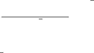
It can be shown mathematically that the following two equations produce values of

a and b that, when inserted in the general equation, describe the best-ﬁt straight line:

b =

∑

−(

∑

)(

∑

)

∑

−(

∑

)

and

a =

Y −bX

RELATING A MEASUREMENT TO ANOTHER MEASUREMENT 207

where n = the number of elements in the sample, X

= the X value for the ith

element, and Y

= the Y value for the ith element.

Since the summations involved in the equation for b are complex, it is perhaps

worth explaining the operation in detail. For the ﬁrst term in the numerator of the

fraction, n

∑

, we multiply the X value for each element in the sample by the Y

value for the same element, then sum up these n products, and multiply the total by

n. For the second term in the numerator, (

∑

)(

∑

), we sum up all nXvalues,

sum up all nY values, and multiply the two totals together. For the ﬁrst term in the

denominator, n

∑

, we square each X value, sum up all these squares, and multiply

the total by n. And for the second term in the denominator, (

∑

)

, we sum up all

the X values and then square the total. Having arrived at a value for b,derivingthe

value of a is quite easy by comparison. We simply subtract the product of b times

the mean of X from the mean of Y.

There are computational shortcuts for performing these cumbersome calcula-

tions, but in fact there is little likelihood that any reader of this book will perform

a regression analysis without a computer, so we will not take up space with these

shortcut calculations. Neither will we laboriously work these equations through by

hand to arrive at the actual numbers for our example. This example has been per-

formed the way everyone now can fully expect to perform a regression analysis, by

computer. The point of including the equations here, then, is not to provide a means

of calculation but instead to provide insight into what is being calculated and thus

into what the results may mean.

PREDICTION

Once we have the values of a and b, of course, we can specify the equation relating

X and Y and, by plugging in any two numbers as given X values, determine the

corresponding Y values and use these two points to draw the best-ﬁt straight line

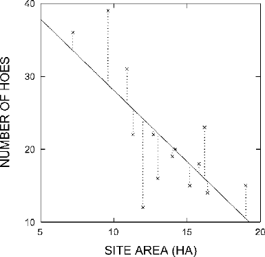
on the graph. If we do this for the data from Table

15.1, we get the result shown in

Fig.

15.6. The values obtained in this regression analysis are

a = 47.802

and

b = −1.959

Thus the equation relating X to Y is

Y = −1.959X + 47.802

Number of hoes =(−1.959 ×Site area)+47.802

208 CHAPTER 15

Figure 15.6. The best-ﬁt straight line for the points from Fig. 15.1.

This equation literally enables us to “predict” how many hoes there will be per 100

artifacts collected if we know the site area. For example, if the site area is 15.2 ha,

we predict

Y =(−1.959)(15.2)+47.802 = 18.03

Thus, if the relationship between X and Y described by the regression equation

holds true, a site with an area of 15.2 ha should yield 18.03 hoes in a collection

of 100 artifacts. There actually was a site in the original data set with an area of

15.2 ha, and the collection of 100 artifacts from that site had 15 hoes. For this site,

then, reality fell short of the predicted number of hoes by 3.03. Thus the residual for

that site is −3.03, representing a bit of variation unpredicted or “unexplained” by

the regression equation. (The name “residual” is used because residuals represent

unexplained or leftover variation.) The prediction based on the regression equation

is, however, a better prediction than we would otherwise be able to make. Without

the regression analysis our best way to predict how many hoes would be collected

at each site would be to use the mean number of hoes for all sites, or 21.57 hoes.

This would have meant an error of 6.57 hoes in the case of the 15.2 ha site. In this

instance, then, the regression equation has enabled us to predict how many hoes

would be found on the basis of site area more accurately than we could if we were

unaware of this relationship. This will not necessarily be true for every single case

in a regression analysis, but it will be true on average.

Regression analysis, then, has helped us to predict or “explain” some of the vari-

ation in number of hoes collected per 100 artifacts. It has, however, still left some

of the variation “unexplained.” We do not know why the 15.2 ha site had 3.03 fewer

hoes than we expected. The residuals represent this unexplained variation, a subject

to which we shall return below.

RELATING A MEASUREMENT TO ANOTHER MEASUREMENT 209

HOW GOOD IS THE BEST FIT?

We know that the equation

Y = −1.959X + 47.802

represents the best-ﬁt straight line for our example data, so that the sum of the

squares of the residuals is the lowest possible (for straight-line equations). These

residuals are shown with dotted lines in Fig.

15.6. We notice immediately that some

of them are quite large. Although the best-ﬁt straight line does help us predict or

explain some of the variability in number of hoes collected, it clearly does not ﬁt

the data as well as we might have hoped. It would be useful for us to be able to say

just how good a ﬁt it is, and the very process of determining the best-ﬁt straight line

provides us with a way to do so. Since the best-ﬁt straight line is the one for which

the sum of the squares of the residuals is least, then the lower the sum of the squares

of the residuals, the better the ﬁt. The sum of the squares of the residuals becomes a

measure of how well the best-ﬁt straight line ﬁts the points in the scatter plot.

The sum of the squares of the residuals, of course, can never be less than 0,

because there will never be a negative number among the squared residuals that are

summed. (Even negative residuals have positive squares.) The sum of the squares

of the residuals will only be 0 when all the residuals are 0. This only happens when

all the points lie exactly on the straight line and the ﬁt is thus perfect. There is no

ﬁxed upper limit on the sum of the squares of the residuals, however, because it

depends on the actual values taken by Y. It would be useful if we could determine

this upper limit because then we would know just where, between the minimum

and maximum possible values, a particular sum of squared residuals lay. We could

then determine whether the best-ﬁt straight line really was closer to the best of all

possible ﬁts (a value of zero for the sum of the squares of the residuals) or the worst

of all possible ﬁts (whatever that maximum value for the sum of the squares of the

residuals might be). It turns out that the maximum value the sum of the squares

of the residuals can have is the sum of the squares of the deviations of Y from its

mean. (The sum of the squares of the deviations of Y from its mean is, of course,

the numerator in the calculation of the variance of Y –thatis,

∑



−Y



.) Thus the

ratio

(sum of the squares of residuals)

∑



−Y



ranges from zero to one. Its minimum value of zero indicates a perfect ﬁt for the

best-ﬁt straight line because it only occurs when all the residuals are zero. Its max-

imum value of one indicates the worst possible ﬁt because it occurs when the sum

of the squares of the residuals is as large as it can be for a given set of values of Y

(that is, equal to

∑



−Y



This ratio, then, enables us to say, on a scale of zero to one, how good a ﬁt the

best-ﬁt straight line is. Zero means a perfect ﬁt, and one means the worst possible

ﬁt. It is easier intuitively to use a scale on which one is best and zero is worst, so

210 CHAPTER 15

we customarily reverse the scale provided by this ratio by subtracting the ratio from

one. (If this does not make intuitive good sense to you, try it with some numbers.

For example, 0.2 on a scale from zero to one becomes 0.8 on a scale from one to

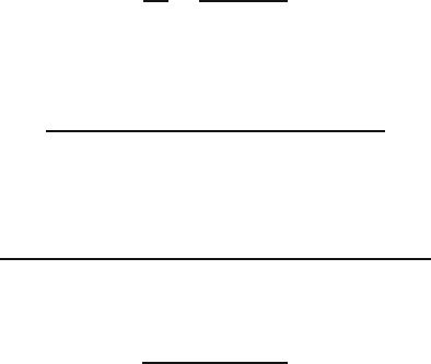
zero.) This ratio, when subtracted from one, is called r

,and

= 1 −

(sum of the squares of residuals)

∑



−Y



The ratio, r

, amounts to a ratio of variances. The denominator is the original vari-

ance in Y (omitting only the step of dividing by n – 1) and the numerator is the

variance that Y has from the best-ﬁt straight line (again omitting only the step of

dividing by n – 1). Including the step of dividing by n – 1 would have no effect on

the result since it would occur symmetrically in both numerator and denominator.

If the variation from the best-ﬁt straight line is much less than the original vari-

ation of Y from its mean, then the value of r

is large (approaching one) and the

best-ﬁt straight line is a good ﬁt indeed. If the variation from the best-ﬁt straight

line is almost as large as the original variation of Y from its mean, then the value

of r

is small (approaching zero) and the best-ﬁt straight line is not a very good

ﬁt at all. Following from this logic, it is common to regard r

as a measure of the

proportion of the total variation in Y explained by the regression. This also follows

from our consideration of the residuals as variation unexplained or unpredicted by

the regression equation. All this, of course, amounts to a rather narrow mathematical

deﬁnition of “explaining variation,” but it is useful nonetheless within the constraints

of linear regression. For our example, r

turns out to be 0.535, meaning that 53.5%

of the variation in number of hoes per collection of 100 artifacts is explained or

accounted for by site area. This is quite a respectable amount of variation to account

for in this way.

More commonly used than r

, is its square root, r, which is also known as

Pearson’s r or the product-moment correlation coefﬁcient or just the correlation

coefﬁcient. We speak, then, of the correlation between two measurement variables

as a measure of how good a ﬁt the best-ﬁt straight line is. Since r

ranges from zero

to one, then its square root must also range from zero to one. While r

must always

be positive (squares of anything always are), r can be either positive or negative.

We give r the same sign as b, the slope of the best-ﬁt straight line. As a conse-

quence, a positive value of r corresponds to a best-ﬁt straight line with a positive

slope and thus to a positive relationship between X and Y , that is, a relationship in

which as X increases Y also increases. A negative value of r corresponds to a best-

ﬁt straight line with a negative slope and thus to a negative relationship between X

and Y, that is, a relationship in which as X increases Y decreases. The correlation

coefﬁcient r, then, indicates the direction of the relationship between X and Y by its

sign, and it indicates the strength of the relationship between X and Y by its abso-

lute value on a scale from zero for no relationship to one for a perfect relationship

(the strongest possible). In our example, r = −0.731, which represents a relatively

strong (although negative) correlation.

RELATING A MEASUREMENT TO ANOTHER MEASUREMENT 211

SIGNIFICANCE AND CONFIDENCE

Curiously enough, the question of signiﬁcance has not arisen up to now in Chap-

ter

15. The logic of our approach to relating two measurement variables has been

very different from our approach to relating two categorical variables or one mea-

surement variable and one categorical variable. Through linear regression, however,

we have arrived at a measure of strength of the relationship, r, the correlation coef-

ﬁcient. This measure of strength is analogous to V, the measure of strength of

association between two categorical variables. It is analogous to the actual differ-

ences between means of subgroups in analysis of variance as an indication of the

strength of relation between the dependent and independent variables. We still lack,

however, a measure of the signiﬁcance of the relationship between two measure-

ments. What we seek is a statistic analogous to χ

for two categorical variables, or

t or F for a categorical variable and a measurement – a statistic whose value can be

translated into a statement of how likely it is that the relation we observe is no more

than the effect of the vagaries of sampling.

Much of our discussion about arriving at the best-ﬁt straight line and providing

an index of how good a ﬁt it is centered on variances and ratios of variances. This

sounds a great deal like analysis of variance, and indeed it is by calculating F as a

ratio of variances that we arrive at the signiﬁcance level in a regression analysis. In

analysis of variance we had

F =

d. f.

whichistosay

F =

(sum of squares between groups

d. f.)

(sum of squares within groups

d. f.)

In regression analysis we have

F =

(sum of squares explained by regression

d. f.)

(sum of squares unexplained by regression

d. f.)

This is equivalent to

F =

(1 −r

)

(n −2)

In our example, F = 13.811, with an associated probability of 0.003. As usual,

very low values of p in signiﬁcance tests indicate very signiﬁcant results. There are

several ways to think about the probability values in this signiﬁcance test. Perhaps

the clearest is that this result indicates a probability of 0.003 of selecting a random

sample with a correlation this strong from a population in which these two variables

were unrelated. That is, there are only three chances in 1,000 that we could select a

212 CHAPTER 15

sample of 14 sites showing this strong a relation between area and number of hoes

from a population of sites in which there was no relation between area and number

of hoes. Put yet another way, there is only a 0.3% chance that the relationship we

observe in our sample between site area and number of hoes reﬂects nothing more

than the vagaries of sampling. If we are willing to treat these 14 sites as a random

sample of Oasis phase sites from the R´ıo Seco valley, then, we are 99.7% conﬁdent

in asserting that larger Oasis phase sites in the R´ıo Seco valley tend to have fewer

hoes per 100 artifacts on their surfaces.

As usual, signiﬁcance probabilities can be used to tell us how likely it is that the

observation of interest in our sample (in this case the relationship between site area

and number of hoes) does not actually exist in the population from which the sample

was selected. We can also discuss regression relationships in terms of conﬁdence, in

a manner parallel to our earlier use of error ranges for different conﬁdence levels. In

this case, instead of an individual estimate ± an error range, it is useful to think of

just what the relationship between the two variables is likely to be in the population

from which our sample came. We know from the signiﬁcance probability obtained in

our example that it is extremely unlikely that there is no relationship at all between

site area and number of hoes in the population of sites from which our 14 sites are a

sample. The speciﬁc relationship expressed by the regression equation derived from

analysis of our sample is our best approximation of what the relationship between

site area and number of hoes is in the population. But, as in all our previous experi-

ence with samples, the speciﬁc relationship observed in the sample may well not be

exactly the same as the speciﬁc relationship that exists in the population as a whole.

Most likely the regression equation we would obtain from observing the entire pop-

ulation (if we could) would be similar to the one we have derived from analysis of

the sample. It is less likely (but still possible) that the relationship in the population

as a whole is rather different from the relationship observed in the sample. And, as

Be Careful How You Say It

We might report the results of the example regression analysis in the text by

saying, “For Oasis phase sites in the R´ıo Seco valley there is a moderately

strong correlation between site area (X) and number of hoes per collection

of 100 artifacts (Y) (r = −.731, p = .003, Y = −1.959X + 47.802).” This

makes clear what relationship was investigated; it lets the reader know what

signiﬁcance test was used; it provides the results in terms of both strength

and signiﬁcance; and it states exactly what the best-ﬁt linear relationship is.

Like “signiﬁcance,” the word “correlation” has a special meaning in statistics

that differs from its colloquial use. It refers speciﬁcally to Pearson’s r and

other analogous indexes of the relationship between two measurements. Just

as “signiﬁcant” should not be used in statistical context to mean “important”

or “meaningful,” “correlated” should not be used in statistical context to refer

simply to a general correspondence between two things.

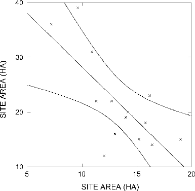
RELATING A MEASUREMENT TO ANOTHER MEASUREMENT 213

Figure 15.7. The best-ﬁt straight line with its 95% conﬁdence zone.

the signiﬁcance probability has already told us, it is extremely unlikely (only three

chances in 1,000) that there is no relationship at all between site area and hoes in

the population.

This range of possible relationships that might exist in the population our sam-

ple came from, and their varying probabilities, can be depicted graphically as in

Fig.

15.7. It is neither very practical nor very enlightening to discuss the calcula-

tion of the curves that delimit this 95% conﬁdence region. In practice, it is almost

unimaginable now to produce such a graph except by computer, so we will con-

centrate on what the graph tells us. The 95% conﬁdence region, which includes the

best-ﬁt straight line for our sample in its center, depicts the zone within which we

have 95% conﬁdence that the best-ﬁt straight line for the population lies. There is

only a 5% chance that the best-ﬁt straight line for the population of sites from which

our sample of 14 was selected (if we could observe the entire population) would not

lie entirely between the two curves. Determination of this conﬁdence region, then,

enables us to think usefully about the range of possible relationships between site

area and number of hoes likely to exist in the population from which our sample

came. Depiction of this conﬁdence region relates to the signiﬁcance probability in

the same way that our previous use of error ranges for different conﬁdence levels

related to parallel signiﬁcance tests.

ANALYSIS OF RESIDUALS

The regression analysis described in the example used above has enabled us to

explain a portion of the variation in number of hoes per collection of 100 arti-

facts. One possible interpretation of these results is that larger settlements contained

214 CHAPTER 15

Table 15.2. Hoes at Oasis Phase Sites in the R´ıo Seco Valley: Predictions and Residuals

Site area Number of hoes Number of hoes predicted Residual

(ha) per 100 artifacts by regression on site area number of hoes

19.0 15 10.59 4.41

16.4 14 15.68 −1.68

15.8 18 16.86 1.14

15.2 15 18.03 −3.03

14.2 20 19.99 0.01

14.0 19 20.38 −1.38

13.0 16 22.34 −6.34

12.7 22 22.93 −0.93

12.0 12 24.30 −12.30

11.3 22 25.67 −3.67

10.9 31 26.45 4.55

9.6 39 29.00 10.00

16.2 23 16.07 6.93

7.2 36 33.70 2.30

larger numbers of craft workers and elite residents and fewer farmers. Thus hoes

were scarcer in the artifact assemblages at the larger sites. (We would presumably

have had something like this in mind in the ﬁrst place or we would not likely have

been interested in investigating the relationship between site area and number of

hoes at all. We would also presumably have provided the additional evidence and

argumentation necessary to make this a truly convincing interpretation.)

Since the regression analysis has explained part of the variation in number of

hoes, it has also left another part of this variation unexplained. This unexplained

variability is made speciﬁc in the form of the residuals. The 15.2-ha site that we

discussed, for instance, actually had 3.03 fewer hoes than the regression analysis

led us to expect, based on the size of the site. This 3.03 is its residual, or leftover

variation. For each site there is, likewise, a residual representing how much the

observed number of hoes differed from the predicted number of hoes. Table

15.2

provides the original data together with two new items. For each site, the number of

hoes per collection of 100 artifacts predicted on the basis of the regression equation

relating number of hoes to site area is listed. Then comes the residual for each site

(that is the number of hoes actually collected minus the number predicted by the

regression equation).

In examining the residuals, we note as expected that some sites had considerably

fewer hoes than we predicted and some had substantially more than we predicted.

We can treat these residuals as another variable whose relationships can be explored.

In effect, the regression analysis has created a new measurement – the variation in

number of hoes unexplained by site size. We can deal with this new measurement

just as we would deal with any measurement we might make. We would begin to

explore it by looking at a stem-and-leaf plot and perhaps a box-and-dot plot. We