Davidson K.R., Donsig A.P. Real Analysis with Real Applications

Подождите немного. Документ загружается.

6.3 Riemann Integration 153

(b) Suppose that f(0) = 0, and let g(0) = f

(0) and g(x) = f(x)/x for x > 0. Show

that g is continuous and strictly increasing.

L. Suppose that f is a continuous function on R such that lim

h→0

f(x + h) − f (x − h)

= 0

for every x ∈ R. Prove that f is constant.

HINT: Fix ε > 0. For each x, ﬁnd a δ > 0 so that |f(x + h) − f(x − h)| ≤ εh for

0 ≤ h ≤ δ. Let ∆ be the supremum of all such δ. Show that ∆ = ∞.

M. Find a discontinuous function f on R such that lim

h→0

f(x + h) − f (x − h)

= 0 for

every x ∈ R.

N. Suppose that f is C

on [0, ∞), and let C = {x : f

(x) = 0}.

(a) If C is bounded, show that lim

x→∞

f(x) exists or is ±∞.

(b) If C is unbounded and lim

x∈C, x→∞

f(x) = L, prove that lim

x→∞

f(x) = L.

HINT: Compare f (x) to the value of f at the nearest critical points on either side.

O. Suppose that f is C

on [0, ∞), and lim

x→∞

f(x)+f

(x) = 0. Prove that lim

x→∞

f(x) = 0.

HINT: Use the previous exercise.

6.3. Riemann Integration

We turn now to integration. A crucial point of this section is that the word

derivative never appears—well, only twice. An integral is deﬁned as a limit related

to area, not as an antiderivative. In the next section, we establish the Fundamen-

tal Theorem of Calculus, which shows that integration and differentiation are, in

some sense, inverse operations. This theorem sometimes allows us to replace the

complicated limit calculation with a simpler calculation using differential calculus.

However, we cannot prove this theorem until we ﬁrst deﬁne clearly what an integral

is. This necessarily involves a limiting process.

Besides carefully deﬁning integrals, we will establish that two classes of func-

tions are always integrable: continuous functions and monotone functions. This is

sufﬁcient for many applications. There are more powerful kinds of integrals that, at

the price of much more technical machinery, can integrate more functions and sat-

isfy very strong limit theorems. We describe one approach to such “better, stronger,

faster” integrals in Section 9.6. But for the applications we study in this book, the

Riemann integral will do all we need.

The goal is to deﬁne the Riemann integral of a function f deﬁned on an inter-

val [a, b]. The idea is simple and geometric. Chop the interval up into a partition

consisting of a number of smaller subintervals. Approximate f as well as possible

above and below by functions that are constant on each subinterval. This approx-

imates the region bounded by f above and below by the union of a number of

rectangles. We know the areas of these upper and lower approximations, and they

are called the upper and lower sums for this partition. For a ‘reasonable’ function,

154 Differentiation and Integration

we will show that as the partition is made ﬁner and ﬁner, these upper and lower es-

timates will converge to a common value. This limit, when it exists, will be called

the integral of f from a to b.

Now we make precise what we just described.

6.3.1. DEFINITION. Let f be a bounded function deﬁned on an interval [a, b].

A partition of [a, b] is a ﬁnite set P = {a = x

< x

< . . . < x

n−1

< x

= b}. Set

∆

= x

−x

j−1

and deﬁne the mesh of a partition P as mesh(P ) = max

1≤j≤n

∆

For each interval [x

j−1

, x

] of this partition, we deﬁne the maximum and minimum

of f on this interval by

(f, P ) = sup

j−1

≤x≤x

f(x) and m

(f, P ) = inf

j−1

≤x≤x

f(x).

Then deﬁne the upper and lower sums of f with respect to the partition P by

U(f, P ) =

j=1

(f, P )∆

and L(f, P ) =

j=1

(f, P )∆

If, in addition, we are given a set of points X = {x

: 1 ≤ j ≤ n}, where

∈ [x

j−1

, x

] for 1 ≤ j ≤ n, we deﬁne the Riemann sum

I(f, P, X) =

j=1

f(x

)∆

A partition R is a reﬁnement of a partition P provided that P ⊂ R. If P and

Q are two partitions, then R is a common reﬁnement of P and Q provided that

P ∪ Q ⊂ R.

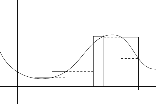
a = x

= b

FIGURE 6.6. Example of upper and lower sums

6.3 Riemann Integration 155

Figure 6.6 illustrates upper and lower sums. We always have

L(f, P ) ≤ I(f, P, X) ≤ U (f, P ).

If R reﬁnes P , then each interval I of R is contained in an interval J of P . Now

it is evident that if I is a subinterval of J, then the maximum over I is at most the

corresponding max over J, and the minimum over I is at least the corresponding

min over J. This is the only depth to the following estimate.

6.3.2. LEMMA. If R is a reﬁnement of P, then

L(f, P ) ≤ L(f, R) ≤ U (f, R) ≤ U(f, P ).

PROOF. Consider an interval [x

j−1

, x

] of P , and note that this may be subdivided

by R into x

j−1

= t

< ··· < t

= x

. As noted previously, we have the estimate

for k + 1 ≤ i ≤ l,

(f, P ) = inf

j−1

≤x≤x

f(x) ≤ inf

i−1

≤t≤t

f(t) = m

(f, R)

and

(f, R) = sup

i−1

≤t≤t

f(t) ≤ sup

j−1

≤x≤x

f(x) = M

(f, P ).

Thus

(f, P )(x

− x

j−1

) ≤

i=k+1

(f, R)(t

− t

i−1

)

and

i=k+1

(f, R)(t

− t

i−1

) ≤ M

(f, P )(x

− x

j−1

Summing over all the intervals of P now yields

L(f, P ) ≤ L(f, R) ≤ U (f, R) ≤ U(f, P ).

We easily obtain another useful inequality from this:

6.3.3. COROLLARY. If P and Q are any two partitions of [a, b],

L(f, P ) ≤ U (f, Q).

PROOF. Let R be the common reﬁnement of P and Q. Then by the previous

lemma, L(f, P ) ≤ L(f, R) ≤ U (f, R) ≤ U(f, Q). ¥

In particular, we see that the set of numbers {L(f, P )} is bounded above by

any U(f, Q). Hence by the completeness of R, sup

L(f, P ) is deﬁned. Moreover,

sup

L(f, P ) ≤ U (f, Q) for every partition Q. Therefore, inf

U(f, P ) is deﬁned

and sup

L(f, P ) ≤ inf

U(f, P ).

156 Differentiation and Integration

6.3.4. DEFINITION. Deﬁne L(f ) = sup

L(f, P ) and U (f) = inf

U(f, P ).

As pointed out previously, L(f ) ≤ U(f). A bounded function f on a ﬁnite inter-

val [a, b] is called Riemann integrable if L(f) = U (f). In this case, we write

f(x) dx for the common value.

We establish Riemann’s Condition for integrability, which follows easily from

our deﬁnition.

6.3.5. RIEMANN’S CONDITION.

Let f(x) be a bounded function on [a, b]. The following are equivalent:

(1) f is Riemann integrable.

(2) For each ε > 0, there is a partition P so that U(f, P ) − L(f, P ) < ε.

PROOF. Assume that (2) holds. Then for any ε > 0, using the given P we have

L(f, P ) ≤ L(f) ≤ U(f ) ≤ U(f, P ).

Hence 0 ≤ U(f ) − L(f) ≤ U(f, P ) − L(f, P ) < ε. So U(f) = L(f) and (1)

holds.

If f is Riemann integrable, let L = L(f) = U (f). Let ε > 0. We can ﬁnd two

partitions P

and P

so that U(f, P

) < L + ε/2 and L(f, P

) > L − ε/2. Let P

be their common reﬁnement, P

∪ P

. By Lemma 6.3.2,

L −

< L(f, P ) ≤ U(f, P ) < L +

and so U(f, P ) − L(f, P ) < ε, proving (2). ¥

6.3.6. COROLLARY. Let f be a bounded real-valued function on [a, b]. If there

is a sequence of partitions of [a, b], P

, so that

lim

n→∞

U(f, P

) − L(f, P

) = 0,

then f is Riemann integrable. Moreover, if X

is any choice of points x

n,j

selected

from each interval of P

, then

lim

n→∞

I(f, P

, X

) =

f(x) dx.

PROOF. Riemann’s condition is veriﬁed by hypothesis. Hence by Theorem 6.3.5,

f is Riemann integrable. Therefore, both I(f, P

, X

) and

f(x) dx lie in the

intervals [L(f, P

), U(f, P

)]. Consequently,

I(f, P

, X

) −

f(x) dx

≤ U (f, P

) − L(f, P

6.3 Riemann Integration 157

The right-hand side is less than any given ε > 0 for n sufﬁciently large, and there-

fore lim

n→∞

I(f, P

, X

) =

f(x) dx. ¥

A typical choice is the evenly spaced partition

P = {x

= a + j(b − a)/n : 0 ≤ j ≤ n}.

However, it is sometimes convenient to choose a partition better suited to the func-

tion f such as the next example, where constant ratios are used rather than constant

widths.

6.3.7. EXAMPLE. Consider the function f(x) = x

on [a, b], where p 6= −1

and 0 < a < b. Take the partition P

= {a = x

< x

< . . . < x

= b}, where

= a

j/n

for 0 ≤ j ≤ n.

To keep the notation under control, let R = (b/a)

1/n

. For example, x

= aR

and ∆

= x

−x

j−1

= aR

j−1

(R−1). Since f is monotone increasing when p ≥ 0,

we easily compute

(f, P

) = inf

j−1

≤x≤x

f(x) = x

j−1

= a

p(j−1)

and

(f, P

) = sup

j−1

≤x≤x

f(x) = x

= a

= R

(f, P

When p < 0, m

and M

are reversed. The details of this case are left to the reader.

So for p > 0, we have U(f, P

) = R

L(f, P

) and

L(f, P

) =

j=1

(f, P

)∆

j=1

p(j−1)

j−1

(R − 1)

= a

p+1

(R − 1)

n−1

j=0

(p+1)j

Summing the geometric series and rearranging, we have

L(f, P

) = a

p+1

(R − 1)

n(p+1)

− 1

p+1

− 1

= a

p+1

(R − 1)

p+1

− 1

p+1

− 1

= (b

p+1

− a

p+1

)

R − 1

p+1

− 1

We will take a limit as n → +∞. To show the role of n clearly, we set r =

and h = 1/n, so that R = r

1/n

= r

. The key is to recognize the limit as the

158 Differentiation and Integration

computation of two derivatives.

lim

n→∞

L(f, P

) = (b

p+1

− a

p+1

) lim

n→∞

1/n

− 1

(p+1)/n

− 1

= (b

p+1

− a

p+1

) lim

h→0

− 1

(p+1)h

− 1

= (b

p+1

− a

p+1

)

x=0

(p+1)x

x=0

= (b

p+1

− a

p+1

)

logr

(p + 1) log r

p+1

− a

p+1

p + 1

Since U(f, P

) =

p/n

L(f, P

) has the same limit, we conclude that

p+1

− a

p+1

p + 1

≤ L(f ) ≤ U(f) ≤

p+1

− a

p+1

p + 1

So this function is Riemann integrable with

dx =

p+1

− a

p+1

p + 1

Given the many concepts we have already presented using an ²–δ formulation,

it is natural to ask if Riemann integrable functions can be described in this way.

There is such a formulation, given as Condition (3) in the next theorem, but it is

harder to verify than the deﬁnition or Riemann’s condition. Condition (4) shows

that we can skip the step of ﬁnding the maximum and minimum values on each

interval and instead use the Riemann sum for arbitrarily chosen points. Frequently,

the choice of the left or right endpoint of the interval is both natural and convenient.

6.3.8. THEOREM. Let f (x) be a bounded function on [a, b]. The following are

equivalent:

(1) f is Riemann integrable.

(2) For each ε > 0, there is a partition P so that U(f, P ) − L(f, P ) < ε.

(3) For every ε > 0, there is a δ > 0 so that every partition Q such that

mesh(Q) < δ satisﬁes U(f, Q) − L(f, Q) < ε.

(4) For every ε > 0, there is a δ > 0 so that every partition Q such that

mesh(Q) < δ and every choice of set X = {x

: 1 ≤ j ≤ n}, where

∈ [x

j−1

, x

] satisﬁes

I(f, Q, X) −

f(x) dx

< ε.

PROOF. We have already veriﬁed that (1) and (2) are equivalent. Clearly, (3) im-

plies (2). Let us prove that (1) implies (3).

If f is Riemann integrable, let L = L(f) = U (f). Let ε > 0. We can ﬁnd two

partitions P

and P

so that U(f, P

) < L + ε/4 and L(f, P

) > L − ε/4. Let P

6.3 Riemann Integration 159

be their common reﬁnement, P

∪ P

. By Lemma 6.3.2,

L −

< L(f, P ) ≤ U(f, P ) < L +

Let n be the number of points in P , and set δ =

8nkfk

∞

, where kfk

∞

sup{|f(x)| : x ∈ [a, b]}.

Now suppose that Q is any partition with mesh(Q) < δ. Deﬁne R = P ∪Q to

be the common reﬁnement of P and Q. By Lemma 6.3.2 again, we obtain

L −

< L(f, R) ≤ U (f, R) < L +

The intervals of R coincide with the intervals of Q except for at most n−1 intervals

of Q which are split in two by the points in P . Thus in the sums determining

L(f, R) and L(f, Q), all the terms are the same except for terms from these n − 1

intervals. Fix one of these intervals of Q, say I. The inﬁmum of f over I is no

smaller than −kfk

∞

, and the inﬁmum of f over any subinterval of R contained in

I is no more than +kfk

∞

. Adding up the differences over the n −1 such intervals

of Q, the total can be no more than

L(f, R) − L(f, Q) ≤ (n − 1)(2kfk

∞

) mesh(Q)

< 2nkf k

∞

8nkfk

∞

Hence L(f, Q) > L −

. Likewise, U(f, Q) < L +

. So U(f, Q) − L(f, Q) < ε

and (3) is valid.

To see that (3) implies (4), ﬁx a partition Q and a set X = {x

: 1 ≤ j ≤ n},

where x

∈ [x

j−1

, x

]. Then

L(f, Q) ≤ I(f, Q, X) ≤ U (f, Q) < L(f, Q) + ε.

Since L(f, Q) ≤

f(x) dx ≤ U(f, Q) < L(f, Q) + ε also, it follows that

I(f, Q, {x

}) −

f(x) dx

< ε.

Conversely, if (4) holds, then every choice of X satisﬁes this inequality for

ε/3. If x

satisfy f(x

) = inf

j−1

≤x≤x

f(x), then I(f, Q, X) = L(f, Q). Hence

L(f, Q) −

f(x) dx

< ε/3. If the inﬁmum is not attained, then we can choose

X so that f(x

) are sufﬁciently close to this inﬁmum to obtain the inequality

L(f, Q) −

f(x) dx

< ε/2. The details of this argument are left as an ex-

ercise. Similarly,

U(f, Q) −

f(x) dx

< ε/2. Hence U(f, Q) − L(f, Q) < ε.

So (3) holds. ¥

160 Differentiation and Integration

Using Riemann’s condition, we can now show that many functions are inte-

grable.

6.3.9. THEOREM. Every monotone function on [a, b] is Riemann integrable.

PROOF. We will assume that f is monotone increasing, but the reader can easily

convert this to a proof for decreasing functions. Consider the uniform partition P

given by x

= a +

j(b−a)

for 0 ≤ j ≤ n. Notice that m

(f, P ) = f(x

j−1

) and

(f, P ) = f(x

). Thus we obtain a telescoping sum

U(f, P ) − L(f, P ) =

j=1

f(x

)

b − a

−

j=1

f(x

j−1

)

b − a

f(b) − f(a)

(b − a)

It is evident that given any ε > 0, we may choose an integer n sufﬁciently large,

namely n >

f(b)−f(a)

(b−a)ε

−1

, so that U(f, P )−L(f, P ) < ε. This veriﬁes

Riemann’s condition, and therefore f is integrable. ¥

6.3.10. THEOREM. Every continuous function on [a, b] is integrable.

PROOF. This result is deeper than the result for monotone functions because we

must use Theorem 5.5.9 to deduce that a continuous function f on [a, b] is uni-

formly continuous.

Let ε > 0. By uniform continuity, there is a δ > 0 so that for x, y ∈ [a, b]

with |x − y| < δ, we have |f(x) − f (y)| < ε/(b − a). Let P be any partition

with mesh(P ) < δ. Then for any points x, y in a common interval [x

j−1

, x

], we

have |f(x) − f(y)| < ε/(b − a). Hence M

(f, P ) − m

(f, P ) ≤ ε/(b − a).

Consequently,

U(f, P ) − L(f, P ) =

j=1

(f, P ) − m

(f, P )

∆

≤

b − a

j=1

∆

= ε.

Thus Riemann’s condition is satisﬁed, and f is Riemann integrable. ¥

6.3.11. EXAMPLE. There do exist functions that are not Riemann integrable.

For example, consider f : [0, 1] → R deﬁned by

f(x) =

(

1 if x ∈ Q

0 if x /∈ Q.

6.3 Riemann Integration 161

Let P be any partition. Notice that M

(f, P ) = 1 and m

(f, P ) = 0 for all j. Thus

we see that

U(f, P ) =

j=1

− x

j−1

= 1 and L(f, P ) = 0.

This holds for all P . Thus it follows that L(f) = 0 and U (f) = 1, and so f is not

Riemann integrable. The reason for this failure is that f is discontinuous at every

point in [0, 1].

6.3.12. EXAMPLE. On the other hand, there are discontinuous functions that

are Riemann integrable. For example, the characteristic function

(.5,1]

is Riemann

integrable on [0, 1] because it is monotone. However, the discontinuity is rather

banal.

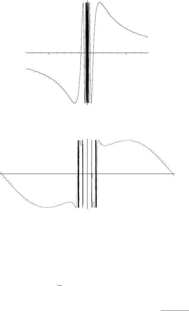
Consider f(x) = sin(1/x) on (0, 1], and set f(0) = 0. This function has

a nasty discontinuity at the origin, as shown in Figure 6.7. But it turns out that

providedthat the function remains bounded, even bad discontinuities at a fewpoints

do not prevent integrability.

Let ε > 0 be given. We will choose a partition P with x

= ε/4. Notice that

since f is continuous on [ε/4, 1], it is integrable there. Thus there is a partition

Q = {x

= ε/4 < ··· < x

= 1} of [ε/4, 1] with

U(f|

,1]

, Q) − L(f |

,1]

, Q) <

Now take P = {0}∪Q as a partition of [0, 1]. Then since sin(1/x) oscillates wildly

between ±1 near x = 0, it follows that M

(f, P ) = 1 and m

(f, P ) = −1. So

U(f, P ) = ∆

+ U (f|

,1]

, Q) =

+ U (f|

,1]

, Q)

and

L(f, P ) = −∆

+ L(f |

,1]

, Q) = −

+ L(f |

,1]

, Q).

Therefore,

U(f, P ) − L(f, P ) =

+ U (f|

,1]

, Q) − L(f |

,1]

, Q) < ε.

So f is integrable.

A similar analysis applies to the function g(x) = sin(csc(1/x)), which is

graphed in Figure 6.8. This function behaves badly at those x where csc(1/x)

is undeﬁned, namely where sin(1/x) = 0. Since sin(t) = 0 for t = nπ, these

discontinuities occur at x = 1/(nπ) for n ≥ 1 and at the endpoint x = 0 where

g is undeﬁned. Moreover, on an interval around one of these discontinuities, say

[1/(xπ), 1/((x+1)π)], where x = n+1/2, g has, qualitatively, the same behaviour

as sin(1/x) has around the origin.

Nonetheless, this function is integrable on [0, 1]. A small choice of x

takes

care of all but ﬁnitely many of these bad points, much as before. The remaining

points can be handled by ensuring that the partition contains each remaining dis-

continuity in a very small interval. The details are left to the reader as an exercise.

162 Differentiation and Integration

–2 2

FIGURE 6.7. The graph of sin(1/x).

FIGURE 6.8. Partial graph of sin(csc(1/x)) from −π to π.

Exercises for Section 6.3

A. (a) Compute the upper Riemann sum for f(x) = x

−1

on [a, b] using the partition

= {x

= a(b/a)

j/n

: 0 ≤ j ≤ n}.

(b) Evaluate the integral

dx. HINT: Recognize lim

n→∞

U(f, P

) as a derivative.

B. (a) Compute the upper Riemann sum for f(x) = x

on [a, b] using the uniform parti-

tion P

= {x

= a + j(b − a)/n : 0 ≤ j ≤ n}. HINT:

j=1

n(n+1)(2n+1)

(b) Hence evaluate the integral

dx.

C. Show that if a function f : [a, b] → R is Lipschitz with constant C, then for any

partition P of [a, b], we have U (f, P ) − L(f, P ) ≤ C(b − a) mesh(P ).