Das Sh.P. Statistical Physics of Liquids at Freezing and Beyond
Подождите немного. Документ загружается.

A8.2 Field-theoretic treatment of the DDFT model 441
We now go back to the full equation (A8.2.40) for the dynamics of the density correlation
function. Following the above scheme, we introduce an irreducible memory function M
I
with the equation
∂
∂t
G
ρρ
(q, t) =−
2
q
G
ρρ
(q, t) +
t
0
dt
M
I
(q, t − t
)
∂
∂s
G
ρρ
(q, s)
.
(A8.2.53)
Direct comparison with eqn. (A8.2.40) shows that M
I
satisfies
t
0
dt
M
I
(q, t − t
)
∂G
ρρ
(q, s)
∂s
=
t
0
dt
−2
q
˜
ˆρ ˆρ
(q, t − t
) +
ˆρ
ˆ
θ
(q, t − t
)
∂
∂t
G
ρρ
(q, t
)
+
t
0
dt
˜
ˆρ ˆρ
(q, t − t
)
t
0
ds M
I
(q, t
− s)
∂
∂s
G
ρρ
(q, s). (A8.2.54)
Laplace transformation of eqn. (A8.2.54) gives the following self-consistent relation
for M
I
:
M
I
(q, z) =
R
(q, z) +M
I
(q, z)
˜
ˆρ ˆρ
(q, z), (A8.2.55)
where we have defined
R
(q, t) as
R
(q, t) =
−2
q
˜
ˆρ ˆρ
(q, t) +
ˆρ
ˆ
θ
(q, t)
. (A8.2.56)
In the time space this reduces to the relation for the irreducible part M
I
:
M
I
(q, t) =
R
(q, t) +
t
0
ds M
I
(q, t − s)
ˆρ ˆρ
(q, s). (A8.2.57)
To summarize, the dynamics of the density correlation function G
ρρ
is obtained from
the equation of motion (A8.2.53) in terms of the irreducible kernel M
I
which satisfies
eqn. (A8.2.57). To lowest order
M
I
(q, t) =
R
(q, t). (A8.2.58)
The equation satisfied by the density correlation function is therefore obtained as
∂
∂t
G
ρρ
(q, t) =−
2
q
G
ρρ
(q, t) +
t
0
dt
R
(q, t − t
)
∂
∂s
G
ρρ
(q, s)
= 0.
(A8.2.59)
The above equation represents the feedback mechanism of MCT if we express
R
self-
consistently in terms of the density correlation function G
ρρ
.Fromeqn. (A8.2.59) it fol-
lows that slowing the dynamics of the density correlation function increases
R
, eventually
causing the ENE transition, beyond which the density correlation function is frozen and
R
(q, 0) diverges. In other words, a 1/z pole in G
ρρ
(z) self-consistently gives rise to the
442 Appendix to Chapter 8
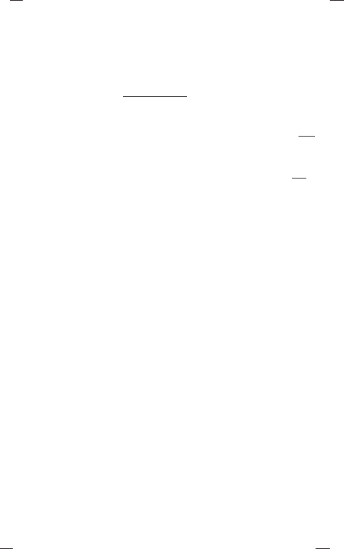
Fig. A8.1 The one-loop diagrams at O(k
B
T ) for the self-energy
ˆv
i
ˆv
j
. The lines joining at both
ends with the vertices represent fully renormalized correlation or response functions as labeled. The
corresponding three-leg vertices are both given by (7.3.61).
1/z pole in
R
(z). Kim and Kawasaki (2008) reported that at one-loop level even the wave-
vector dependence of
R
(in its self-consistent form) controlling the ENE transition point
is identical to that predicted from the simplified treatment reported in eqns. (8.1.139) and
(8.1.140).
A8.3 The one-loop result for
ˆ
v
ˆ
v
(0, 0)
The cutoff function γ is also obtained self-consistently in terms of the hydrodynamic
correlation functions. We state the results in terms of the kernel in time γ(q, t), where
γ(q, z) =
∞
o
dt e
izt
γ(q, t). (A8.3.1)
γ(q, z) is expressed as the sum of two parts, γ
L
and γ
T
, referring to the longitudinal and
transverse parts in the isotropic fluid, respectively. Since the cutoff function γ is defined
in the hydrodynamic limit as q
2
γ(q, z) ∼ q
ˆvρ
, we evaluate the former in terms of the
self-energy
ˆv ˆv
using the relation (7.3.55). From the one-loop diagrams for the self-energy
ˆv ˆv
shown in Fig. A8.1 we obtain the one-loop contributions as (Das and Mazenko, 1986)
γ
L
(q, t) =
1
2n
0
dk
(2π)
3
u
k
u
k
+
u
1
k
1
S(k)S(k
1
)
S(q)
˙
φ(k
1
, t)
˙
φ(k, t), (A8.3.2)
γ
T
(q, t) =
1
2n
0
dk
(2π)
3
(1 − u
2
)
S(k
1
)
S(q)
φ(k
1
, t)φ
T
(k, t),
where
˙
φ is the time derivative of the function φ, k
1
≡ q − k, u =
ˆ
q ·
ˆ
k, and u
1
=
ˆ
q ·
ˆ
k
1
.
The hatted quantity denotes the corresponding unit vector. This one-loop-order result for
the cutoff function is valid only in the hydrodynamic limit.

9
The nonequilibrium dynamics
In the present chapter we discuss the nonequilibrium dynamics and aging (Struik, 1978)
in structural glasses. The nonequilibrium state has been studied quite extensively through
computer simulations and application of mean-field models. We discuss here the char-
acterization of the nonequilibrium state through plausible extensions of the equilibrium-
thermodynamics description and consider possible applications of the new results obtained
for the dynamics. In this regard the model based on the similarity between structural glasses
and spin glasses has proved to be very useful for understanding the simulation results
for the structural glass. Indeed, such findings further consolidate the underlying similarity
between disordered systems with and without intrinsic disorder.
9.1 The nonequilibrium state
A characteristic behavior of the nonequilibrium state is the violation of the fluctuation–
dissipation theorem (FDT) discussed in Chapter 1. In the following we first consider the
FDT violation seen in simulation studies and in certain mean-field theoretical models.
9.1.1 A generalized fluctuation–dissipation relation
The fluctuating-hydrodynamics model discussed in the previous chapter refers to fluctua-
tions around the equilibrium state for which the FDT equation
R(t, t
) =
1
k
B
T
∂C(t, t
)
∂t
linking the correlation function C(t, t
) and the response function R(t, t
) holds. (See
eqn. (1.3.72) in Chapter 1 for this standard result of equilibrium statistical mechanics.)
For simplicity we omit the subscripts indicating the dynamic variables associated with
C and R. For glassy dynamics the FDT is generalized in a parametric form by defining a
quantity X (t, t
) (for t > t
)as
R(t, t
) =
X (t, t
)
k
B
T
∂C(t, t
)
∂t
. (9.1.1)
443

444 The nonequilibrium dynamics
The crucial assertion here is that, taking the similarity to the mean-field structural-glass
(SG) models, in the limit of long times t
, t →∞, X (t, t
) is expressed as a function of
the correlation function C(t, t
) only, i.e., X (t, t
) ≡ x[C(t, t
)] (say). Equation (9.1.1) is
expressed in terms of the integrated response function M defined as
M(t, t
) =
t
t
ds R(t, s) =−
1
k
B
T
1
C
x(c)dc, (9.1.2)
where we have used a normalization C(t, t ) = 1. It is clear that a plot of −k
B
TM vs. C
has slope −x(C). When the FDT is obeyed,
k
B
TM(t − t
) = C(t − t
) − 1, (9.1.3)
and hence the slope x =−1. A more general form of x(C) corresponds to violation of
the FDT. In the parametric representation in terms of x(C) the violation of the FDT is
presented in terms of correlation windows rather than time windows.
9.1.2 Computer-simulation studies
The aging behavior in a supercooled liquid was studied by Kob and Barrat (1998, 2000)
using molecular-dynamics simulations. These authors used a binary mixture of Lennard-
Jones particles (BMLJ) – referred to as the Kob–Anderson mixture introduced earlier in
Section 4.3.1. Binary systems continue to remain in the liquid state without crystallization
and are suitable for studying the dynamics below the freezing transition. We had earlier dis-
cussed (see Section 8.2.3) computer-simulation studies of the equilibrium dynamics of the
BMLJ system and their use in testing the predictions of the mode-coupling theory. These
studies are done mainly in the temperature range 0.45 < T < 0.8. The nonequilibrium
dynamics was obtained with the simulation of 1000 particles at constant volume V = L
3
in cubic box length L = 9.4. The aging behavior was studied in terms of the two-point cor-
relation functions C(τ +t
w
, t
w
) for different waiting times t
w
. Following results from the
mean field theories and experimental data of spin glasses, the behavior of the correlation
function in the aging regime is tested for the form C(t
w
+τ ;t
w
) ∼ C
A
[h(t
w
+τ)/h(t
w
)],
where h(x ) is a monotonically increasing function of its argument x. The correlation func-
tion depends on two times in the absence of time-translational invariance (which holds
for short times). Thus the τ and t
w
dependences of the correlation function in the aging
regime enter only through the combination h(t
w
+ τ)/h(t
w
). The form of the function
h(t) can be used to distinguish between different theoretical models to describe the aging
dynamics, e.g., the droplet model of Fisher and Huse (1986, 1988) for spin glasses predicts
h(t) ∼ log(t). It was argued (Müssel and Rieger, 1998) that the Lennard-Jones model
showed this type of aging dynamics. Aging in the BMLJ system was considered by first
equilibrating the system in the high-temperature phase at a temperature T
i
> T
c
and then
quenching at time t = 0 to a temperature T
f
< T
c
. Following the quench, the system was
allowed to evolve for a waiting time t
w
, after which the measurements of the quantities of
9.1 The nonequilibrium state 445
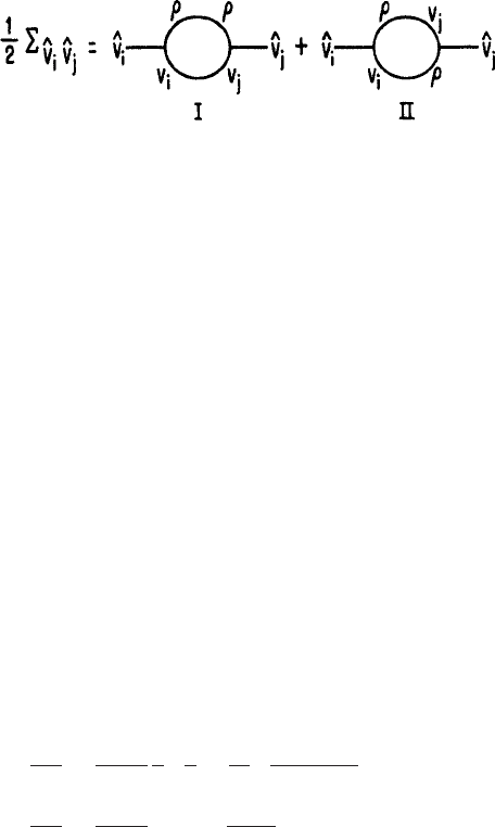
Fig. 9.1 The two time correlation function as a function of the variable [h(τ + t
w
)/ h(t
w
) − 1]
for different wave vectors k = 3.0, 7.23, and 12.5. In each case the waiting times t
w
=
0, 10, 100, 1000, 10 000, and 63 100 time units are considered. The function h(t) was chosen to make
the curves for k = 7.23 collapse at long times and its t dependence is shown in the inset. Reproduced
from Kob and Barrat (2000).
c
Europhysics Journal B.
interest were started. Figure 9.1 shows the scaling of the correlation functions for differ-
ent values of t
w
=0, 10, 100, 1000, 10 000, and 63 100 time units at three different wave
vectors, k = 3.0, 7.23, and 12.5. In the inset of the figure the h(t) function corresponding
to the structure factor peak, i.e., k = 7.23, is shown. This h(t) is chosen to make the best
collapse of the different t
w
data at this wave vector. To a first approximation h(t) is close to
a logarithm, but significant deviations occur. For wave vectors different from the structure-
factor peak, the curves for the different t
w
values do not collapse nicely at long times. This
indicates that the scaling function h(t) depends on the corresponding observable – which
in this case is density fluctuations at a particular wave length.
Let us now consider the violation of the FDT as seen in the computer simulations of
the supercooled liquids in the nonequilibrium state. For the structural glasses the corre-
lation and response functions for the liquid have been studied extensively by Kob and
Barrat (2000) using molecular-dynamics simulations of binary mixtures of the Lennard-
Jones (BMLJ) system. The linear response function is studied by adding a small fictitious
“charge” κ =±1 randomly to each particle and defining the observable,
O
k
(t) =
i
κ
i
cos(k · R
i
(t)), (9.1.4)
where R
i
(t) is the position of the ith particle at time t. An additional term of the form
H ≡ h
0
i
κ
i
cos(k · R
i
) (9.1.5)
is added to the Hamiltonian to represent coupling of O to the field h
0
. In the computer
simulation the liquid is quenched at t = 0 from the initial high temperature T
i
to a low
temperature T
f
, and the evolution of the system is followed by keeping the field h
0
off until
time t = t
w
.Attimet = t
w
+ τ the average of the variable O
k
(over different realizations
446 The nonequilibrium dynamics
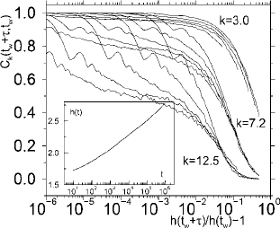
Fig. 9.2 A parametric plot of the integrated response function M(t
w
+ τ, t
w
) and the correlation
function C (t
w
+τ,t
w
) for wave vector k = 7.25, at the quenched temperature (see the text) T
f
= 0.3:
circles, t
w
= 1000; and triangles, t
w
= 10 000. Time and wave vector are expressed in the Lennard-
Jones units (see the text). The straight lines have slopes −1.0and−0.45. Reproduced from Kob and
Barrat (1999).
c
Europhysics Letters.
of the random distributions of κ) in the presence of the conjugate field h
0
(which couples
to O
k
) is denoted in terms of the integrated response function M(τ + t
w
, t
w
):
O
k
(τ + t
w
, t
w
)=h
0
t
w
τ +t
w
R(τ +t
w
, s)ds = h
0
M(τ +t
w
, t
w
). (9.1.6)
The correlation and response functions obtained are presented in Fig. 9.2 in a paramet-
ric plot of −k
B
TM(t, t
) vs. C(t, t
) over different ranges of C (Kob and Barrat, 1997).
This is shown here for T
f
=0.3 referring to the temperature to which the system is ini-
tially quenched. For short times (C close to 1) the data for different t
collapse onto
a single curve of slope −1, showing that the FDT holds. For smaller values of C the
slope of this curve is not unity, indicating FDT violation. The corresponding values of
the parameter X ≡m obtained by Kob and Barrat for three temperatures T
f
=0.4, 0.3, and
0.1 were independent of the wave vector and were compatible with a linear dependence of
m on T
f
.
One-component Lennard-Jones systems have also been simulated for studying FDT vio-
lation. The problem of crystallization of a one-component system makes it difficult to study
it in the supercooled state. Di Leonardo et al. (2000) studied the FDT in a system of 256
particles interacting with a Lennard-Jones potential modified by inclusion of a small many-
body term in its potential energy to inhibit crystallization. The off-equilibrium dynamics
of the system was studied after sudden isothermal (at temperature T ) compressions from
well-equilibrated liquid configurations towards the glassy state. The response functions
9.1 The nonequilibrium state 447
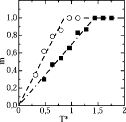
Fig. 9.3 The temperature dependence of the FDT-violation factor in the nonequilibrium state for two
densities of a one-component LJ system: nσ
3
= 1.14 (open circles) and nσ
3
= 1.24 (filled squares).
Fits shown with dashed lines give the corresponding effective temperatures T
eff
(see the text) as 0.86
and 1.43, respectively. Reproduced from Di Leonardo et al. (2000).
c
American Physical Society.
were computed by introducing dynamic variables similar to O
k
discussed above for the
BMLJ case. The generalized FDT was studied and the violation parameter m was obtained
as a function of temperature T . The result for the FDT-violation parameter is shown in
Fig. 9.3. At low temperature, m(T ) is proportional to T , crossing over to m =1 at a char-
acteristic temperature T
c
. The linear temperature dependence of m below a characteristic
temperature conforms to the predictions in the one-step replica-symmetry-breaking sce-
nario proposed for the spin glasses (Mézard et al., 1987). An interesting question in this
regard is that of how the temperature T
c
for the liquid compares with other characteris-
tic temperatures of the dynamics of structural glasses. The calorimetric glass-transition
temperature T
g
at which the time scale of equilibration of the supercooled liquid crosses
the laboratory time scale indicates the liquid falling out of equilibrium. On the other hand,
from consideration of the FDT, above T
c
the system falls out of equilibrium and this is
expected to correspond to the calorimetric glass-transition temperature. In the case of the
MD simulation of a BMLJ system Kob and Barrat (2000) report a crossover tempera-
ture T
c
≈0.7 that is much higher than T
g
. In the one-component Lennard-Jones system
the agreement between these two temperatures is much better. The crossover temperature
from liquid- to solid-like behavior has been obtained by analyzing the temperature depen-
dence of the potential energy. In the glassy state the time scale of relaxation becomes so
large that the liquid behaves like an amorphous solid. Equilibrium MD studies show that
the potential energy for the liquid crosses over from T
5/3
behavior (liquid-like) to linear
dependence (solid-like) at a temperature close to T
c
.
The FDT violation in supercooled liquids has also been studied using (see Section 4.3.1)
an approach based on inherent structures in the potential-energy landscape (PEL). A new
temperature T
int
is identified for the nonequilibrium system. The free energy of the liquid
is obtained here as a sum of configurational and vibrational parts,
f (e
IS
) = e
IS
− T
int
s
conf
+ f
vib
(e
IS
, T ), (9.1.7)
448 The nonequilibrium dynamics
where e
IS
is the energy of the local minima corresponding to a basin of attraction in the
PEL, s
conf
counts the number of minima with energy e
IS
, and f
vib
is the average free
energy of a basin of depth e
IS
. T denotes the temperature of the bath (which is attained
by the fast degrees of freedom) and T
int
is the Lagrange multiplier used to extremize f .
In equilibrium T
int
=T , the temperature of the bath. From the landscape studies of the
typical fragile BMLJ system it was shown (Sciortino and Tartaglia, 2001) that T
int
is close
to T/m, where m is denoted as the FDT violation parameter. A steady perturbation applied
to the system at t = t
w
is given by the H
(t) =−V
0
Bδ(t − t
w
) due to the coupling of
the dynamic variable B with a constant field. The Fourier transform of the density of the
particles of species α at wave vector k is obtained as ρ
α
k
=
5
N
α
i=1
e
ik.R
α
i
/
√
N .LetB =
ρ
α
k
+ρ
α∗
k
be identified with the real part of ρ
α
k
. Since the applied field is constant here, the
linear response function will be proportional to the perturbed value of the coupled variable
at time τ, i.e., ρ
α
k
(τ ). The corresponding correlation function is denoted by S
αα
k
(τ ) =
ρ
α
k
(τ )ρ
α
k
(0)
0
. The correlation and response functions are obtained at different values of
τ corresponding to two waiting times t
w
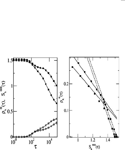
=1024 and 16 384. In Fig. 9.4 the behaviors of
the correlation and response functions are displayed, demonstrating the violation of the
FDT. In equilibrium m =1, whereas for the glassy state m < 1. For strong liquids such as
Fig. 9.4 FDT violation using PEL study. Left: the time dependences of the response function (see
the text for its definition) ρ
α
k
(τ ) (open symbols) and the correlation function S
αα
k
(τ ) (filled symbols)
for the two waiting times t
w
=1024 (circles) and t
w
=16 384 (squares). Right: a parametric plot
of correlation and response functions similar to Fig. 9.2. The solid lines have slope proportional
to 1/k
B
T
int
with T
int
(see the text for its definition) respectively corresponding to the two inherent
structures characterized by e
IS
(t
w
=1024) =−7.576 and e
IS
(t
w
=16 384) =−7.602, both with the
same bath temperature T =0.25. The two dashed lines correspond to the equilibrated system with
slope proportional to 1/k
B
T . The wave vector corresponds to k = 6.7. From Sciortino and Tartaglia
(2001).
c
American Physical Society.
9.2 The effective temperature 449
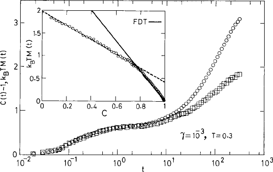
Fig. 9.5 The quantity [1 −C
k
(t)]/T involving the correlation function (squares) and the integrated
response function M
k
(t) (circles) vs. time t. The temperature and shear rates are shown in the legend.
The two curves overlap when the FDT is satisfied for small t and for larger values of the correlation
functions. The inset shows a plot of C and M similar to Fig. 9.1. From Berthier and Barrat (2002).
c
American Institute of Physics.
silica (Scala et al., 2003), however, the unexpected result m > 1 was found in the out-of-
equilibrium state.
The out-of-equilibrium state of the liquid can also be obtained by applying a steady-state
perturbation to the system, e.g., applying a homogeneous steady shear flow (Berthier and
Barrat, 2002). The steady shear flow is characterized by the corresponding shear rate γ
0
,
which creates a nonequilibrium steady state with time translational invariance. The inverse
of the shear rate γ
−1
0
introduces a time scale and acts as a control parameter in studying
the nonequilibrium state that is similar to the waiting time t
w
in relaxational dynamics. In
Fig. 9.5 the violation of the FDT is shown by comparing the two sides of eqn. (9.1.3) for a
fixed t
w
(i.e., γ
−1
) for the BMLJ system. (See the text near eqns. (4.3.11) and (4.3.12) for
its definition.) The FDT is tested by computing the Fourier transform of the self-part of the
density correlation function C
k
(t) for wave vector k =k
m
e
z
corresponding to the peak of
the structure factor. The liquid is subjected to a steady shear γ =10
−3
expressed in units
of τ
0
for the BMLJ system. The response functions are computed using the random field
defined in eqn. (9.1.4). For small t the FDT is satisfied, but it ceases to hold for large t as
the system enters the aging regime. We discuss such behavior in the context of mean-field
theory below.
9.2 The effective temperature
For a liquid in thermodynamic equilibrium its macroscopic behavior is described in terms
of a small number of thermodynamic variables such as temperature, pressure, volume,
450 The nonequilibrium dynamics
and chemical potential. The statistical-mechanical or microscopic description of a many-
particle system, on the other hand, is formulated in terms of a suitable ensemble of a large
number of similar systems. Each member of this ensemble corresponds to a state of the
system defined by the specific values of the coordinates of the large number of variables for
the constituent particles. For a system in equilibrium the probability density for a particular
member of the corresponding ensemble is characterized in terms of a set of conserved
properties. For a set of conserved quantities A
0
={N , H, P,...}, respectively denoting the
total energy, number of particles, momentum, etc., the corresponding probability density
is given by
f (N , H, P ···) ∼ exp
[
B
0
· A
0
]
, (9.2.1)
as has already been discussed in Section 5.1.2, eqn. (5.1.14). The quantities for B
0
=
{ν, −β, v,...}, in (9.2.1) respectively correspond to the chemical potential, temperature,
and velocity fields etc. describing a particular thermodynamic state of the system. The
equilibrium ensemble describing the possible microscopic states for the system is thus
characterized by a small set of time-independent thermodynamic properties. For systems
that are out of equilibrium, such ideas are extended to modify the definition of ther-
modynamic variables such as temperature. In the local equilibrium ensemble the def-
inition (9.2.1) is extended in terms of time-independent local thermodynamic variables
{ν(r), −β(r), v(r),...}.
For nonequilibrium systems in which such time independence cannot be invoked, devel-
oping an equivalent description is not straightforward. We now require extensions of the
basic ideas applied in formulating the thermodynamics of the equilibrium system. In the
out-of-equilibrium state, the issue of time independence applies only for a class of “fast”
variables that relax over the time scale of observation while the slow variables in the
many-particle system are still evolving with time. For systems showing aging, e.g., for
glassy dynamics, such an approach is very appropriate (Cugliandolo and Kurchan, 1994).
Consider the case of a supercooled liquid that has been quenched from a high to a low
temperature a long time ago and is currently in a weakly perturbed state. The glassy state
has reached relaxation times beyond the laboratory time scales. The driven system reaches
a stationary state after some time and an effective temperature is associated with it. It is
useful to note here that “stationarity” in the present context implies a loss of memory of the
initial conditions. While this property is associated with the equilibrium state of a system,
the converse is not true, i.e., a stationary state does not have all of the other properties of
the Gibbsian ensemble. The time scale associated with the description of such a station-
ary (weakly perturbed) state is related to the strength of the perturbation. For example,
for a system exposed to a steady shear γ
0
, the corresponding time scale is proportional to
γ
−1
0
. The out-of-equilibrium system with extremely slow dynamics is linked to a “temper-
ature” that is suitably defined for the nonequilibrium state. This has been attempted in two
ways.