Cohen I.M., Kundu P.K. Fluid Mechanics
Подождите немного. Документ загружается.

442 Computational Fluid Dynamics
predictor
ρ
∗
i,j
= ρ
n
i,j
−
tU
2x
ρ
n
i+1,j
− ρ
n
i−1,j
+
t
2y
−
(
ρv
)
n
i,j−2
+ 4
(
ρv
)
n
i,j−1
− 3
(
ρv
)
n
i,j
,
(11.145)
corrector
2ρ
n+1
i,j
=ρ
n
i,j
+ ρ
∗
i,j
−
tU
2x
ρ
∗
i+1,j
− ρ
∗
i−1,j
+
t
2y
−
(
ρv
)
∗
i,j−2
+ 4
(
ρv
)
∗
i,j−1
− 3
(
ρv
)
∗
i,j
. (11.146)
In summary, we may organize the explicit MacCormack scheme at each time
step (11.103) to (11.108) into the following six substeps.
Step 1: For 0 i<n
x
and 0 j<n
y
(all nodes):
u
i,j
=
(
ρu
)
n
i,j
%
ρ
n
i,j
,v
i,j
=
(
ρv
)
n
i,j
%
ρ
n
i,j
.
Step 2: For 1 i<n
x
− 1 and 1 j<n
y
− 1 (all interior nodes):
ρ
∗
i,j
= ρ
n
i,j
− a
1
(
ρu
)
n
i+1,j
−
(
ρu
)
n
i,j
− a
2
(
ρv
)
n
i,j+1
−
(
ρv
)
n
i,j
,
(
ρu
)
∗
i,j
=
(
ρu
)
n
i,j
− a
3
ρ
n
i+1,j
− ρ
n
i,j
− a
1
ρu
2
n
i+1,j
−
ρu
2
n
i,j
− a
2
(
ρuv
)
n
i,j+1
−
(
ρuv
)
n
i,j
− a
10
u
i,j
+ a
5
u
i+1,j
+ u
i−1,j
+ a
6
u
i,j+1
+ u
i,j−1
+a
9
v
i+1,j +1
+ v
i−1,j −1
− v
i+1,j −1
− v
i−1,j +1
,
(
ρv
)
∗
i,j
=
(
ρv
)
n
i,j
− a
4
ρ
n
i,j+1
− ρ
n
i,j
− a
1
(
ρuv
)
n
i+1,j
−
(
ρuv
)
n
i,j
− a
2
ρv
2
n
i,j+1
−
ρv
2
n
i,j
− a
11
v
i,j
+ a
7
v
i+1,j
+ v
i−1,j
+ a
8
v
i,j+1
+ v
i,j−1
+ a
9
u
i+1,j +1
+ u
i−1,j −1
− u
i+1,j −1
− u
i−1,j +1
.
Step 3: Impose boundary conditions (at time t
n+1
) for ρ
∗
i,j
,
(
ρu
)
∗
i,j
and
(
ρv
)
∗
i,j
.
Step 4: For 0 i<n
x
and 0 j<n
y
(all nodes):
u
∗
i,j
=
(
ρu
)
∗
i,j
%
ρ
∗
i,j
,v
∗
i,j
=
(
ρv
)
∗
i,j
%
ρ
∗
i,j
.

5. Three Examples 443
Step 5: For 1 i<n
x
− 1 and 1 j<n
y
− 1 (all interior nodes):
2ρ
n+1
i,j
=
ρ
n
i,j
+ ρ
∗
i,j
− a
1
(
ρu
)
∗
i,j
−
(
ρu
)
∗
i−1,j
− a
2
(
ρv
)
∗
i,j
−
(
ρv
)
∗
i,j−1
,
2
(
ρu
)
n+1
i,j
=
(
ρu
)
n
i,j
+
(
ρu
)
∗
i,j
− a
3
ρ
∗
i,j
− ρ
∗
i−1,j
− a
1
ρu
2
∗
i,j
−
ρu
2
∗
i−1,j
− a
2
(
ρuv
)
∗
i,j
−
(
ρuv
)
∗
i,j−1
− a
10
u
∗
i,j
+ a
5
u
∗
i+1,j
+ u
∗
i−1,j
+ a
6
u
∗
i,j+1
+u
∗
i,j−1
+ a
9
v
∗
i+1,j +1
+ v
∗
i−1,j −1
− v
∗
i+1,j −1
− v
∗
i−1,j +1
,
2
(
ρv
)
n+1
i,j
=
(
ρv
)
n
i,j
+
(
ρv
)
∗
i,j
− a
4
ρ
∗
i,j
− ρ
∗
i,j−1
− a
1
(
ρuv
)
∗
i,j
−
(
ρuv
)
∗
i−1,j
− a
2
ρv
2
∗
i,j
−
ρv
2
∗
i,j−1
− a
11
v
∗
i,j
+ a
7
v
∗
i+1,j
+ v
∗
i−1,j
+ a
8
v
∗
i,j+1
+ v
∗
i,j−1
+ a
9
u
∗
i+1,j +1
+u
∗
i−1,j −1
− u
∗
i+1,j −1
− u
∗
i−1,j +1
.
Step 6: Impose boundary conditions for ρ
n+1
i,j
,
(
ρu
)
n+1
i,j
and
(
ρv
)
n+1
i,j
.
The coefficients are defined as,
a
1
=
t
x
,a
2
=
t
y
,a
3
=
t
xM
2
,a
4
=
t
yM
2
,a
5
=
4t
3Re
(
x
)
2
,
a
6
=
t
Re
(
y
)
2
,a
7
=
t
Re
(
x
)
2
,a
8
=
4t
3Re
(
y
)
2
,a
9
=
t
12Rexy
,
a
10
= 2
(
a
5
+ a
6
)
,a
11
= 2
(
a
7
+ a
8
)
.
For coding purposes, the variables u
i,j
(v
i,j
) and u
∗
i,j
(v
∗
i,j
) can take the same storage
space. At the end of each time step, the starting values of ρ
n
i,j
,
(
ρu
)
n
i,j
and
(
ρv
)
n
i,j
will be replaced with the corresponding new values of ρ
n+1
i,j
,
(
ρu
)
n+1
i,j
and
(
ρv
)
n+1
i,j
.
Next we present some of the results and compare them with those in the paper by
Hou et al. (1995) obtained by a lattice Boltzmann method. To keep the flow almost
incompresible, the Mach number is chosen as M = 0.1. Flows with two Reynolds
numbers, Re = ρ
0
UD
/
µ = 100 and 400 are simulated. At these Reynolds numbers,
the flow will eventually be steady. Thus calculations need to be run long enough to
get to the steady state. A uniform grid of 256 by 256 was used for this example.
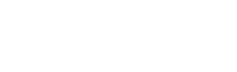
Figure 11.7 shows comparisons of the velocity field calculated by the explicit
MacCormack scheme with the streamlines from Hou (1995) at Re =100 and 400. The
agreement seems reasonable. It was also observed that the location of the center of
the primary eddy agrees even better. When Re =100, the center of the primary eddy
is found at (0.62 ± 0.02, 0.74 ±0.02) from the MacCormack scheme in comparison
with (0.6196, 0.7373) from Hou. When Re =400, the center of the primary eddy is
found at (0.57 ± 0.02, 0.61 ± 0.02) from the MacCormack scheme in comparison
with (0.5608, 0.6078) from Hou.
444 Computational Fluid Dynamics
(a) (b)
Figure 11.7 Comparisons of results from the explicit MacCormack scheme (light gray, velocity vector
field) and those from Hou, et al. (1995) (dark solid streamlines) calculated using a Lattice Boltzmann
Method. (a) Re = 100, (b) at Re = 400.
0
0.2
0.4
0.6
0.8
1
20.4 20.2 0 0.2 0.4 0.6 0.8 1
u
y/D
Explicit MacCormack (Re5100)
Explicit MacCormack (Re5400)
Hou et al. Re5100
Hou et al. Re5400
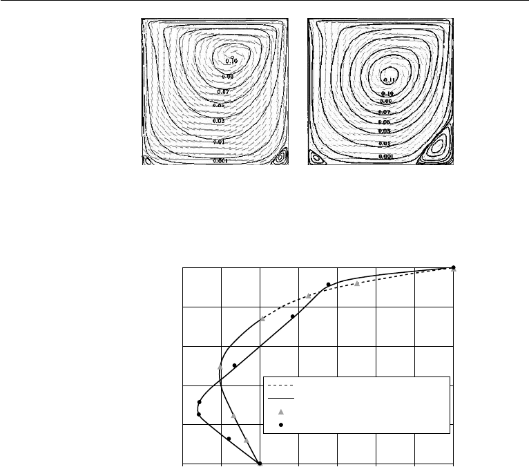
Figure 11.8 Comparison of velocity profiles along a line cut through the center of the cavity (x = 0.5 D)
at Re = 100 and 400.
For a more quantitative comparison, Figure 11.8 plots the velocity profile along
a vertical line cut through the center of the cavity (x = 0.5D). The velocity profiles
for two Reynolds numbers, Re =100 and 400, are compared. The results from the
explicit MacCormack scheme are shown in solid and dashed lines. The data points in
symbols were directly converted from Hou’s paper. The agreement is excellent.
Explicit MacCormack Scheme for Flow Over a Square Block
For the second example, we consider flow around a square block confined between
two parallel plates. Fluid comes in from the left with a uniform velocity profile U, and
the plates are sliding with the same velocity, as indicated in Figure 11.9. This flow
corresponds to the block moving left with velocity U along channel’s center line. In
the calculation we set the channel width H = 3D, the channel length L = 35D with
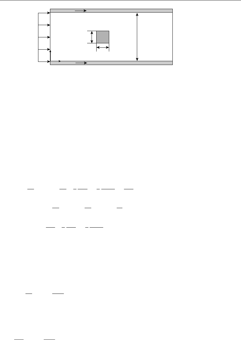
5. Three Examples 445
U
x
y
D
H
D
U
U
Figure 11.9 Flow around a square block between two parallel plates.
15D ahead of the block and 19D behind. The Mach number is set at M =0.05 to
approximate the incompressible limit.
The velocity boundary conditions in this problem are specified as shown in
Figure 11.9, except that at the outflow section, conditions ∂ρu
/
∂x = 0 and ∂ρv
/
∂x =
0 are used. The density (or pressure) boundary conditions are much more compli-
cated, especially on the block surface. On all four sides of the outer boundary (top
and bottom plates, inflow and outflow), the continuity equation is used to update
density as in the previous example. However, on the block surface, it was found
that the conditions derived from the momentum equations give better results. Let us
consider the front section of the block, and evaluate the x-component of the momen-
tum equation (11.97) with u = v = 0,
∂ρ
∂x
= M
2
1
Re
4
3
∂
2
u
∂x
2
+
1
3
∂
2
v
∂x∂y
+
∂
2
u
∂y
2
−
∂
∂x
ρu
2
−
∂
∂y
(
ρvu
)
−
∂
∂t
(
ρu
)
front suface
=
M
2
Re
4
3
∂
2
u
∂x
2
+
1
3
∂
2
v
∂x∂y
.
(11.147)
In (11.147), the variables are non-dimensionalized with the same scaling as the
driven cavity flow problem except that the block size D is used for length. Further-
more, the density gradient may be approximated with a second order backward finite
difference scheme,
∂ρ
∂x
i,j
=
−1
2x
−ρ
i−2,j
+ 4ρ
i−1,j
− 3ρ
i,j
+ O(x
2
). (11.148)
And the second order derivatives for the velocities are expressed as,
∂
2
u
∂x
2
i,j
=
1
x
2
2u
i,j
− 5u
i−1,j
+ 4u
i−2,j
− u
i−3,j
+ O(x
2
) (11.149)
446 Computational Fluid Dynamics
and
∂
2
v
∂x∂y
i,j
=
−1
4xy
−
v
i−2,j +1
− v
i−2,j −1
+ 4
v
i−1,j +1
− v
i−1,j −1
−3
v
i,j+1
− v
i,j−1
+ O
x
2
, xy, y
2
. (11.150)
Substituting (11.148) to (11.150) into (11.147), we have an expression for density
at the front of the block,
ρ
i,j
front
=
1
3
4ρ
i−1,j
− ρ
i−2,j
+
8
9x
M
2
Re
−5u
i−1,j
+ 4u
i−2,j
− u
i−3,j
−
1
18y
M
2
Re
−
v
i−2,j +1
− v
i−2,j −1
+ 4
v
i−1,j +1
− v
i−1,j −1
−3
v
i,j+1
− v
i,j−1
. (11.151)
Similarly at the back of the block,
ρ
i,j
|
back
=
1
3
4ρ
i+1,j
− ρ
i+2,j
−
8
9x
M
2
Re
−5u
i+1,j
+ 4u
i+2,j
− u
i+3,j
−
1
18y
M
2
Re
−
v
i+2,j +1
− v
i+2,j −1
+ 4
v
i+1,j +1
− v
i+1,j −1
−3
v
i,j+1
− v
i,j−1
. (11.152)
At the top of the block, the y-component of the momentum equation should be used,
and it is easy to find that
ρ
i,j
top
=
1
3
4ρ
i,j+1
− ρ
i,j+2
−
8
9y
M
2
Re
−5v
i,j+1
+ 4v
i,j+2
− v
i,j+3
−
1
18x
M
2
Re
−
u
i+1,j +2
− u
i−1,j +2
+ 4
u
i+1,j +1
− u
i−1,j +1
− 3
u
i+1,j
− u
i−1,j
, (11.153)
and finally at the bottom of the block,
ρ
i,j
|
bottom
=
1
3
4ρ
i,j−1
− ρ
i,j−2
+
8
9y
M
2
Re
−5v
i,j−1
+ 4v
i,j−2
− v
i,j−3
−
1
18x
M
2
Re
−
u
i+1,j −2
− u
i−1,j −2
+ 4
u
i+1,j −1
− u
i−1,j −1
−3
u
i+1,j
− u
i−1,j
. (11.154)
5. Three Examples 447
At the four corners of the block, the average values from the two corresponding
sides may be used.
In computation, double precision numbers should be used: otherwise cumulative
round-off error may corrupt the simulation, especially for long runs. It is also helpful
to introduce a new variable for density, ρ
= ρ − 1, such that only the density
variation is computed. For this example, we may extend the FF/BB form of the
explicit MacCormack scheme to have a FB/BF arrangement for one time step and
a BF/FB arrangement for the subsequent time step. This cycling seems to generate
better results.
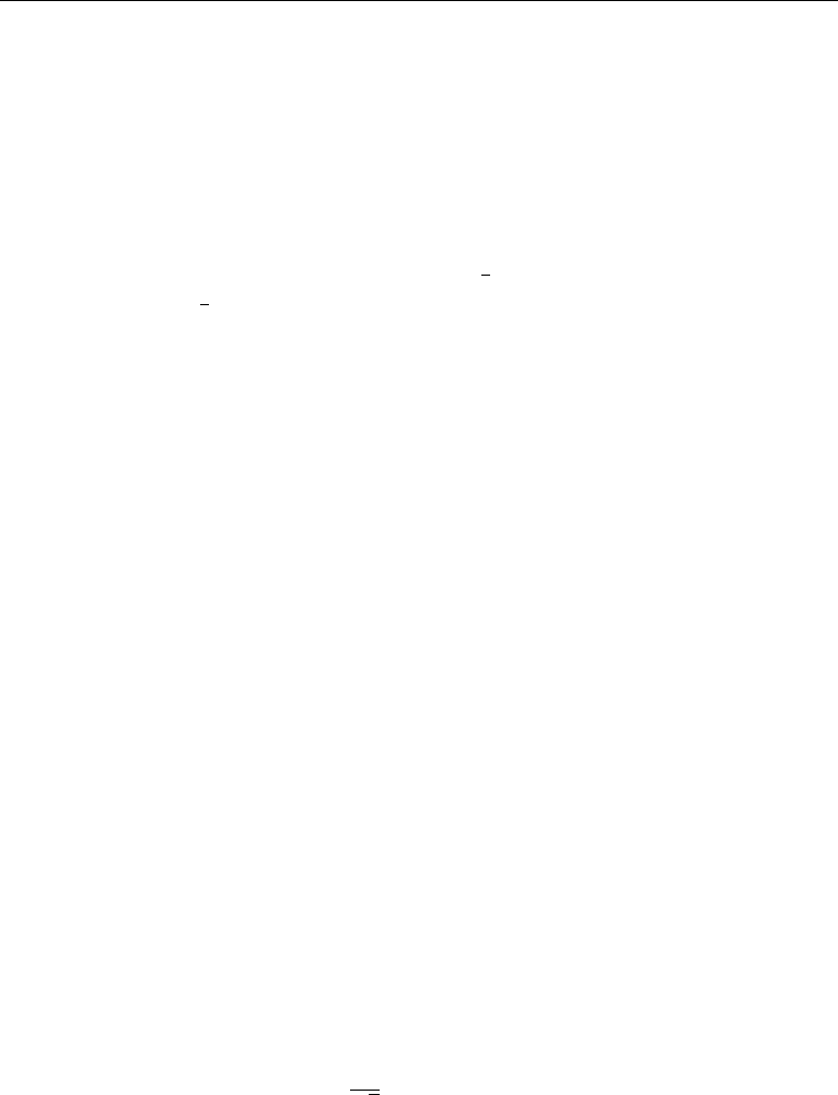
We first plot the drag coefficient, C
D
= Drag
/
(
1
2
ρ
0
U
2
D), and the lift coef-
ficient, C
L
= Lif t
/
(
1
2
ρ
0
U
2
D), as functions of time for flows at two Reynolds
numbers, Re = 20 and 100, in Figure 11.10. For Re = 20, after the initial messy
transient (corresponding to sound waves bouncing around the block and reflecting
at the outflow) the flow eventually settles into a steady state. The drag coefficient
stabilizes at a constant value around C
D
= 6.94 (obtained on a grid of 701x61).
Calculation on a finer grid (1401x121) yields C
D
= 7.003. This is in excellent
agreement with the value of C
D
= 7.005 obtained from an implicit finite element
calculation for incompressible flows (similar to the one used in the next example
in this section) on a similar mesh to 1401x121. There is a small lift (C
L
= 0.014)
due to asymmetries in the numerical scheme. The lift reduces to C
L
= 0.003 on
the finer grid of 1401x121. For Re =100, periodic vortex shedding occurs. Drag
and lift coefficients are shown in Figure 11.10(b). The mean value of the drag coef-
ficient and the amplitude of the lift coefficient are C
D
= 3.35 and C
L
= 0.77,
respectively. The finite element results are C
D
= 3.32 and C
L
= 0.72 under similar
conditions.
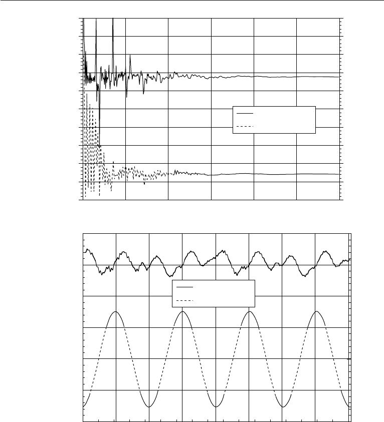
The flow field around the block at Re =20 is shown in Figure 11.11. A steady
wake is attached behind the block, and the circulation within the wake is clearly
visible. Figure 11.12 displays a sequence of the flow field around the block during
one cycle of vortex shedding at Re =100.
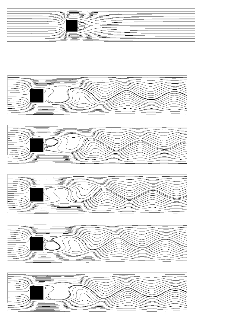
Figure 11.13 shows the convergence of the drag coefficient as the grid spacing
is reduced. Tests for two Reynolds numbers, Re =20 and 100, are plotted. It seems
that the solution with 20 grid points across the block (x = y = 0.05) reasonably
resolves the drag coefficient and the singularity at the block corners does not affect
this convergence very much.
The explicit MacCormack scheme can be quite efficient to compute flows at
high Reynolds numbers where small time steps are naturally needed to resolve high
frequencies in the flow and the stability condition for the time step is no longer too
restrictive. Since with x = y and large (grid) Reynolds numbers, the stability
condition (11.110) becomes approximately,
t
σ
√
2
Mx. (11.155)
As a more complicated example, the flow around a circular cylinder confined between
two parallel plates (the same geometry as the fourth example later in this section) is cal-
culated at Re =1000 using the explicit MacCormack scheme. For flow visualization, a
448 Computational Fluid Dynamics
210
27.5
25
22.5
0
2.5
5
7.5
10
12.5
15
(a)
(b)
0 5 10 15 20 25 30
time
Drag Coefficient
0
0.01
0.02
0.03
0.04
0.05
0.06
0.07
0.08
0.09
0.1
Lift Coefficient
Drag Coefficient
Lift Coefficient
2
1.5
1
0.5
0
20.5
21
Lift Coefficient
3.15
3.2
3.25
3.3
3.35
3.4
3.1
54 .2 55.97 57.74 59.51 61.28 63.05 64.82 66.59 68.36
time
Drag Coefficient
Drag Coefficient
Lift Coefficient
Figure 11.10 Drag and lift coefficients as functions of time for flow over a block. (a) Re =20, on a grid
of 701 ×61, (b) Re = 100, on a grid of 1401 ×121.
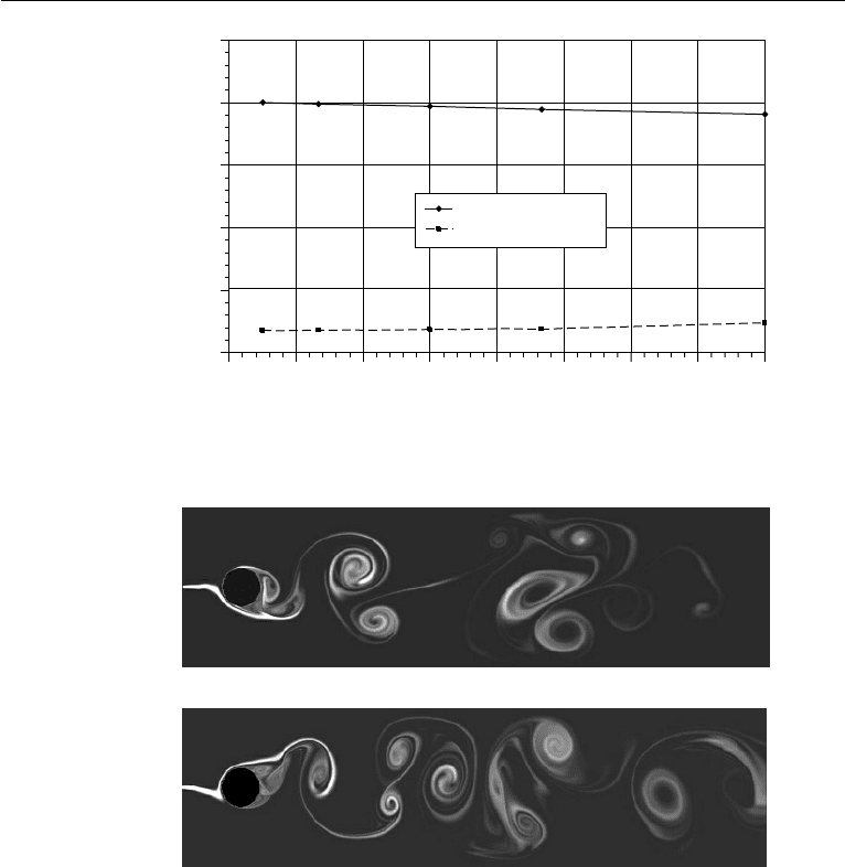
smoke line is introduced at the inlet. Numerically, an additional convection-diffusion
equation for smoke concentration is solved similarly, with an explicit scheme at each
time step coupled with the computed flow field. Two snap shots of the flow field
are displayed in Figure 11.14. In this calculation, the flow Mach number is set at
5. Three Examples 449
Figure 11.11 Streamlines for flow around a block at Re = 20.
(a)
(b)
(c)
(d)
(e)
Figure 11.12 A sequence of flow fields around a block at Re =100 during one period of vortex shedding.
(a) t =40.53, (b) t =41.50, (c) t =42.48, (d) t =43.45, (e) t =44.17.
450 Computational Fluid Dynamics
3
4
5
6
7
8
0.02 0.03 0.04 0.05 0.06 0.07 0.08 0.09 0.1
Grid Spacing
Drag Coefficient
C
D
(Re = 20)
Mean C
D
(Re = 100)
Figure 11.13 Convergence tests for the drag coefficient as the grid spacing decreases. The grid spacing
is equal in both directions x = y, and time step t is determined by the stability condition.
(a)
(b)
Figure 11.14 Smoke lines in flow around a circular cylinder between two parallel plates at Re =1000.
The flow geometry is the same as in the fourth example later in this section.
M =0.3, and a uniform fine grid with 100 grid points across the cylinder diameter
is used.
Finite Element Formulation for Flow Over a Cylinder Confined in a Channel
We next consider the flow over a circular cylinder moving along the center of a
channel. In the computation, we fix the cylinder, and use the flow geometry as shown
in Figure 11.15. The flow comes from the left with a uniform velocity U. Both plates
of the channel are sliding to the right with the same velocity U . The diameter of the
cylinder is d and the width of the channel is W =4d. The boundary sections for the
5. Three Examples 451
x
y
d
U
W
Γ
1
Γ
2
Γ
3
Γ
4
U
U
Γ
5
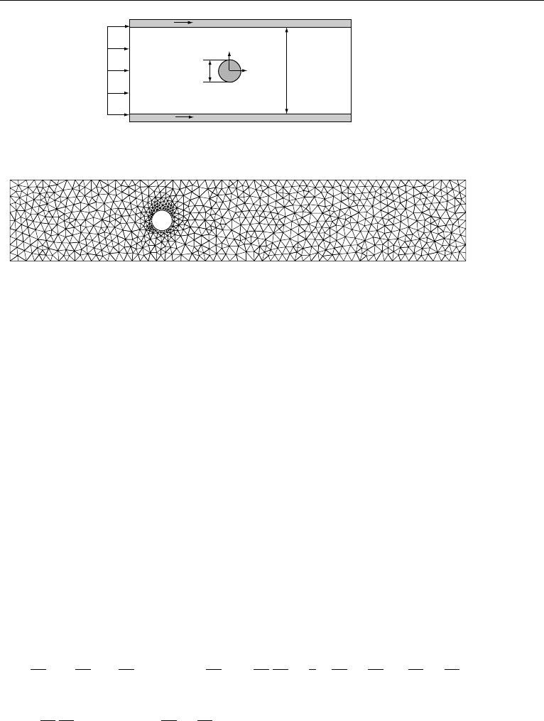
Figure 11.15 Flow geometry of flow around a cylinder in a channel.
Figure 11.16 A finite element mesh around a cylinder.
computational domain are indicated in the figure. The location of the inflow boundary
1
is selected to be at x
min
=−7.5d, and the location of the outflow boundary section
2
is at x
max
= 15d. They are both far away from the cylinder so as to minimize their
influence on the flow field near the cylinder. In order to compute the flow at higher
Reynolds numbers, we relax the assumptions that the flow is symmetric and steady.
We will compute unsteady flow (with vortex shedding) in the full geometry and using
the Cartesian coordinates shown in Figure 11.15.
The first step in the finite element method is to discretize (mesh) the computational
domain described in Figure 11.15. We cover the domain with triangular elements.
A typical mesh is presented in Figure 11.16. The mesh size is distributed in a way
that finer elements are used next to the cylinder surface to better resolve the local flow
field. For this example, the mixed finite element method will be used, such that each
triangular element will have six nodes as shown Figure 11.5a. This element allows
for curved sides that better capture the surface of the circular cylinder. The mesh in
Figure 11.16 has 3320 elements, 6868 velocity nodes, and 1774 pressure nodes.
The weak formulation of the Navier-Stokes equations is given in (11.134) and
(11.135). For this example the body force term is zero, g = 0. In Cartesian coordinates,
the weak form of the momentum equation (11.134) can be written explicitly as
∂u
∂t
+ u
∂u
∂x
+ v
∂u
∂y
·
˜
ud +
2
Re
∂u
∂x
∂ ˜u
∂x
+
1
2
∂u
∂y
+
∂v
∂x
∂ ˜u
∂y
+
∂ ˜v
∂x
+
∂v
∂y
∂ ˜v
∂y
d −
p
∂ ˜u
∂x
+
∂ ˜v
∂y
d = 0, (11.156)
where is the computational domain and
˜
u =
(
˜u, ˜v
)
. Since the variational functions
˜u and ˜v are independent, the weak formulation (11.156) can be separated into two