Cohen I.M., Kundu P.K. Fluid Mechanics

Подождите немного. Документ загружается.

432 Computational Fluid Dynamics

(

ρu

)

n+1

i,j

(

ρu

)

i,j

(

ρu

)

∗

i,j

− c





ρu

+ c



∗

i,j

−



ρu

+ c



∗

i−1,j



− c



(

ρuv

)

∗

i,j

−

(

ρuv

)

∗

i,j−1





∗

i+1,j

− 2u

∗

i,j

+ u

∗

i−1,j



+ c



∗

i,j+1

− 2u

∗

i,j

+ u

∗

i,j−1



+ c



∗

i+1,j +1

+ v

∗

i−1,j −1

− v

∗

i+1,j −1

− v

∗

i−1,j +1



(11.107)

(

ρv

)

n+1

i,j

(

ρv

)

i,j

(

ρv

)

∗

i,j

− c



(

ρuv

)

∗

i,j

−

(

ρuv

)

∗

i−1,j



− c





ρv

+ c



∗

i,j

−



ρv

+ c



∗

i,j−1



+ c



∗

i+1,j

− 2v

∗

i,j

+ v

∗

i−1,j





∗

i,j+1

− 2v

∗

i,j

+ v

∗

i,j−1



+ c



∗

i+1,j +1

+ u

∗

i−1,j −1

− u

∗

i+1,j −1

− u

∗

i−1,j +1



(11.108)

The coefﬁcients are deﬁned as,

t

x

t

y

µt

(

x

)

µt

(

y

)

µt

12xy

(11.109)

In both the predictor and corrector steps the viscous terms (the second-order derivative

terms) are all discretized with centered-differences to maintain second-order accuracy.

For brevity, body force terms in the momentum equations are neglected here.

During the predictor and corrector stages of the explicit MacCormack scheme

(11.103) to (11.108), one-sided differences are arranged in the FF and BB fashion,

respectively. Here, in the notation FF, the ﬁrst F denotes the forward difference in

the x-direction and the second F denotes the forward difference in the y-direction.

Similarly, BB stands for backward differences in both x and y directions. We denote

this arrangement as FF/BB. Similary, one may get BB/FF, FB /BF, BF/FB arrange-

ments. It is noted that some balanced cyclings of these arrangements generate better

results than others.

Tannehill, Anderson and Pletcher (1997) give the following semi-empirical sta-

bility criterion for the explicit MacCormack scheme,

t 



1 + 2









x

y

+ c



x

y

−1

, (11.110)

where σ is a safety factor (≈ 0.9), Re



= min

(

x

µ, ρ

y

)

is the

minimum mesh Reynolds number. This condition is quite conservative for ﬂows with

small mesh Reynolds numbers.

4. Incompressible Viscous Fluid Flow 433

One key issue for the explicit MacCormack scheme to work properly is the

boundary conditions for density (thus pressure). We leave this issue to the next section

where its implementation in two sample problems will be demonstrated.

MAC Scheme

Most of numerical schemes developed for computational ﬂuid dynamics problems can

be characterized as operator splitting algorithms. The operator splitting algorithms

divide each time step into several substeps. Each substep solves one part of the operator

and thus decouples the numerical difﬁculties associated with each part of the operator.

For example, consider a system,

dφ

+ A

(

)

= f, (11.111)

with initial condition φ

(

)

= φ

, where the operator A may be split into two operators

(

)

= A

(

)

+ A

(

)

. (11.112)

Using a simple ﬁrst-order accurate Marchuk-Yanenko fractional-step scheme

(Yanenko, 1971, and Marchuk, 1975), the solution of the system at each time step

n+1

= φ

((

n + 1

)

t

)

(n =0,1, ...) is approximated by solving the following two

successive problems:

n+1

− φ

t

+ A



n+1



= f

n+1

, (11.113)

n+1

− φ

n+1

t

+ A



n+1



= f

n+1

, (11.114)

where φ

= φ

, t = t

n+1

− t

, and f

n+1

+ f

n+1

= f

n+1

= f

((

n + 1

)

t

)

The time discretizations in (11.113) and (11.114) are implicit. Some schemes to be

discussed in what follows actually use explicit discretizations. However, the stability

conditions for those explicit schemes must be satisﬁed.

The MAC (marker-and-cell) method was ﬁrst proposed by Harlow and Welsh

(1965) to solve ﬂow problems with free surfaces. There are many variations of this

method. It basically uses a ﬁnite difference discretization for the Navier-Stokes equa-

tions and splits the equations into two operators

(

u,p

)



(

u ·∇

)

u −

∇



, and A

(

u,p

)



∇p

∇·u



. (11.115)

Each time step is divided into two substeps as discussed in the Marchuk-Yanenko

fractional-step scheme (11.113) and (11.114). The ﬁrst step solves a convection and

diffusion problem, which is discretized explicitly,

n+1

− u

t

+ (u

·∇)u

−

∇

= g

n+1

. (11.116)

434 Computational Fluid Dynamics

In the second step, the pressure gradient operator is added (implicitly) and, at the

same time, the incompressible condition is enforced,

n+1

− u

n+1

t

+∇p

n+1

= 0, (11.117)

and ∇·u

n+1

= 0.

(11.118)

This step is also called a projection step to satisfy the incompressibility condition.

Normally, the MAC scheme is presented in a discretized form. A preferred feature

of the MAC method is the use of the staggered grid. An example of a staggered grid

in two dimensions is shown in Figure 11.4. On this staggered grid, pressure variables

are deﬁned at the centers of the cells and velocity components are deﬁned at the cell

faces, as shown in Figure 11.4.

Using the staggered grid, two components of the transport equation (11.116) can

be written as,

n+1

i+1

2,j

= u

i+1

2,j

−t



∂u

∂x

+ v

∂u

∂y

−

∇



i+1

2,j

+t f

n+1

i+1

2,j

, (11.119)

n+1

i,j+1

= v

i,j+1

−t



∂v

∂x

+ v

∂v

∂y

−

∇



i,j+1

+t g

n+1

i,j+1

, (11.120)

where u =

(

u, v

)

, g =

(

f, g

)



∂u

∂x

+ v

∂u

∂y

−

∇



i+1

2,j

and



∂v

∂x

+ v

∂v

∂y

−

∇



i,j+1

are the functions interpolated at the grid locations for the

1,1

2,1

3,1

1,2

2,2

3,2

1/2,1

3/2,1

5/2,1

1/2,2

3/2,2

5/2,2



1,1/2



2,1/2



3,1/2



3,3/2



1,3/2



2,5/2



1,5/2



3,5/2



2,3/2

Figure 11.4 Staggered grid and a typical cell around p

2,2

4. Incompressible Viscous Fluid Flow 435

x-component of the velocity at

(

i + 1

2,j

)

and for the y-component of the velocity

(

i, j + 1

)

, respectively, and at the previous time t = t

. The discretized form of

(11.117) is

n+1

i+1

2,j

= u

n+1

i+1

2,j

−

t

x



n+1

i+1,j

− p

n+1

i,j



, (11.121)

n+1

i,j+1

= v

n+1

i,j+1

−

t

y



n+1

i,j+1

− p

n+1

i,j



, (11.122)

where x = x

i+1

− x

and y = y

j+1

− y

are the uniform grid spacing in the

x and y directions, respectively. The discretized continuity equation (11.118) can be

written as,

n+1

i+1

2,j

− u

n+1

i−1

2,j

x

n+1

i,j+1

− v

n+1

i,j−1

y

= 0 . (11.123)

Substitution of the two velocity components from (11.121) and (11.122) into the

discretized continuity equation (11.123) generates a discrete Poisson equation for the

pressure,

∇

n+1

i,j

≡

x



n+1

i+1,j

− 2p

n+1

i,j

+ p

n+1

i−1,j



y



n+1

i,j+1

− 2p

n+1

i,j

+ p

n+1

i,j−1



t





n+1

i+1

2,j

− u

n+1

i−1

2,j

x

n+1

i,j+1

− v

n+1

i,j−1

y





. (11.124)

The major advantage of the staggered grid is that it prevents the appearance

of oscillatory solutions. On a normal grid, the pressure gradient would have to be

approximated using two alternate grid points (not the adjacent ones) when a central

difference scheme is used, that is



∂p

∂x



i,j

i+1,j

− p

i−1,j

2x

and



∂p

∂y



i,j

i,j+1

− p

i,j−1

2y

. (11.125)

Thus a wavy pressure ﬁeld (in a zigzag pattern) would be felt like a uniform one

by the momentum equation. However, on a staggered grid, the pressure gradient is

approximated by the difference of the pressures between two adjacent grid points.

Consequently, a pressure ﬁeld with a zigzag pattern would no longer be felt as a

uniform pressure ﬁeld and could not arise as a possible solution. It is also seen that

the discretized continuity equation (11.123) contains the differences of the adjacent

velocity components, which would prevent a wavy velocity ﬁeld from satisfying the

continuity equation.

436 Computational Fluid Dynamics

Another advantage of the staggered grid is its accuracy. For example, the

truncation error for (11.123) is O



x

,y



even though only four grid points

are involved. The pressure gradient evaluated at the cell faces,



∂p

∂x



i+1

2,j

i+1,j

− p

i,j

x

, and



∂p

∂y



i,j+1

− p

i,j

y

, (11.126)

are all second-order accurate.

On the staggered grid, the MAC method does not require boundary conditions for

the pressure equation (11.124). Let us examine a pressure node next to the boundary,

for example p

1,2

as shown in Figure 11.4. When the normal velocity is speciﬁed at the

boundary, u

n+1

2,2

is known. In evaluating the discrete continuity equation (11.123) at

the pressure node

(

1, 2

)

, the velocity u

n+1

2,2

should not be expressed in terms of u

n+1

1/2,2

using (11.121). Therefore p

0,2

will not appear in equation (11.120), and no boundary

condition for the pressure is needed. It should also be noted that (11.119) and (11.120)

only update the velocity components for the interior grid points, and their values at

the boundary grid points are not needed in the MAC scheme. Peyret and Taylor (1983,

chapter 6) also noticed that the numerical solution in the MAC method is independent

of the boundary values of u

n+1

and v

n+1

, and a zero normal pressure gradient on

the boundary would give satisfactory results. However, their explanation was more

cumbersome.

In summary, for each time step in the MAC scheme, the intermediate velocity

components, u

n+1

i+1

2,j

and v

n+1

i,j+1

, in the interior of the domain are ﬁrst evaluated

using (11.119) and (11.120), respectively. Next, the discrete pressure Poisson equation

(11.124) is solved. Finally, the velocity components at the new time step are obtained

from (11.121) and (11.122). In the MAC scheme, the most costly step is the solution

of the Poisson equation for the pressure (11.124).

Chorin (1968) and Temam (1969) independently presented a numerical scheme

for the incompressible Navier-Stokes equations, termed the projection method. The

projection method was initially proposed using the standard grid. However, when it

is applied in an explicit fashion on the MAC staggered grid, it is identical to the MAC

method as long as the boundary conditions are not considered, as shown in Peyret

and Taylor (1983, chapter 6).

A physical interpretation of the MAC scheme or the projection method is that

the explicit update of the velocity ﬁeld does not generate a divergence free velocity

ﬁeld in the ﬁrst step. Thus an irrotational correction ﬁeld, in the form of a velocity

potential which is proportional to the pressure, is added to the nondivergence-free

velocity ﬁeld in the second step in order to enforce the incompressibility condition.

As the MAC method uses an explicit scheme in the convection-diffusion step,

the stability conditions for this method are (Peyret and Taylor, 1983, chapter 6),



+ v



tRe  1, (11.127)

4. Incompressible Viscous Fluid Flow 437

and

4t

Rex

 1, (11.128)

when x = y. The stability conditions (11.127) and (11.128) are quite restrictive

on the size of the time step. These restrictions can be removed by using implicit

schemes for the convection-diffusion step.

-Scheme

The MAC algorithm described in the preceding section is only ﬁrst-order accurate

in time. In order to have a second-order accurate scheme for the Navier-Stokes

equations, the -scheme of Glowinski (1991) may be used. The -scheme

splits each time step symmetrically into three substeps, which are described

here.

• Step 1:

n+θ

− u

θt

−

∇

n+θ

+∇p

n+θ

= g

n+θ

∇

− (u

·∇)u

(11.129)

∇·u

n+θ

= 0. (11.130)

• Step 2:

n+1−θ

− u

n+θ

(1 − 2θ )t

−

∇

n+1−θ

+ (u

∗

·∇)u

n+1−θ

= g

n+1−θ

∇

n+θ

−∇p

n+θ

. (11.131)

• Step 3:

n+1

− u

n+1−θ

θt

−

∇

n+1

+∇p

n+1

= g

n+1

∇

n+1−θ

− (u

n+1−θ

·∇)u

n+1−θ

, (11.132)

∇·u

n+1

= 0. (11.133)

It was shown that when θ = 1 − 1/

√

2 = 0.29289 ...,α + β = 1 and β =

θ/(1 − θ), the scheme is second-order accurate. The ﬁrst and third steps of the

-scheme are identical and are the Stokes ﬂow problems. The second step, (11.131),

represents a nonlinear convection-diffusion problem if u

∗

= u

n+1−θ

. However, it

was concluded that there is practically no loss in accuracy and stability if u

∗

= u

n+θ

is used. Numerical techniques for solving these substeps are discussed in Glowinski

(1991).

438 Computational Fluid Dynamics

Mixed Finite Element Formulation

The weak formulation described in Section 3 can be directly applied to the

Navier-Stokes equations (11.81) and (11.80), and it gives







∂u

∂t

+ u ·∇u − g



ud +





[

]

: D





d −





(

∇·

)

d = 0,

(11.134)





˜p∇·ud = 0, (11.135)

where

u and ˜p are the variations of the velocity and pressure, respectively. The rate

of strain tensor is given by

[

]



∇u +

(

∇u

)



. (11.136)

The Galerkin ﬁnite element formulation for the problem is identical to (11.134)

and (11.135), except that all the functions are chosen from ﬁnite dimensional sub-

spaces and represented in the form of basis or interpolation functions.

The main difﬁculty with this ﬁnite element formulation is the choice of the inter-

polation functions (or the type of the elements) for velocity and pressure. The ﬁnite

element approximations that use the same interpolation functions for velocity and

pressure suffer from a highly oscillatory pressure ﬁeld. As described in the previous

section, a similar behavior in the ﬁnite difference scheme is prevented by introducing

the staggered grid. There are a number of options to overcome this problem with spu-

rious pressure. One of them is the mixed ﬁnite element formulation that uses different

interpolation functions (or ﬁnite elements) for velocity and pressure. The require-

ment for the mixed ﬁnite element approach is related to the so-called Babuska-Brezzi

(or LBB) stability condition, or inf-sup condition. The detailed discussions for this

condition can be found in Oden and Carey (1984). A common practice in the mixed

ﬁnite element formulation is to use a pressure interpolation function that is one order

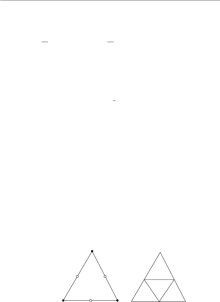
lower than a velocity interpolation function. As an example in two dimensions, a

triangular element is shown in Figure 11.5a. On this mixed element, quadratic inter-

polation functions are used for the velocity components and are deﬁned on all six

nodes, while linear interpolation functions are used for the pressure and are deﬁned

(a) (b)

Figure 11.5 Mixed ﬁnite elements.

4. Incompressible Viscous Fluid Flow 439

on three vertices only. A slightly different approach is to use a pressure grid that is

twice coarser than the velocity one, and then use the same interpolation functions on

both grids (Glowinski, 1991). For example, a piecewise-linear pressure is deﬁned on

the outside (coarser) triangle; while a piecewise-linear velocity is deﬁned on all four

subtriangles, as shown in Figure 11.5b.

Another option to prevent a spurious pressure ﬁeld is to use the stabilized ﬁnite

element formulation while keeping the equal order interpolations for velocity and

pressure. A general formulation in this approach is the Galerkin/least-squares (GLS)

stabilization (Tezduyar, 1992). In the GLS stabilization, the stabilizing terms are

obtained by minimizing the squared residual of the momentum equation integrated

over each element domain. The choice of the stabilization parameter is discussed in

Franca et al. (1992) and Franca and Frey (1992).

Comparing the mixed and the stabilized ﬁnite element formulations, the mixed

ﬁnite element method is parameter free, as pointed out in Glowinski (1991). There

is no need to adjust the stabilization parameters, which could be a delicate problem.

More importantly, for a given ﬂow problem the desired ﬁnite element mesh size

is generally determined based on the velocity behavior (e.g., it is deﬁned by the

boundary or shear layer thickness). Therefore, equal order interpolation will be more

costly from the pressure point of view but without further gains in accuracy. However,

the GLS-stabilized ﬁnite element formulation has the additional beneﬁt of preventing

oscillatory solutions produced in the Galerkin ﬁnite element method due to the large

convective term in high Reynolds number ﬂows.

Once the interpolation functions for the velocity and pressure in the mixed ﬁnite

element approximations are determined, the matrix form of equations (11.134) and

(11.135) can be written as















, (11.137)

where u and p are the vectors containing all unknown values of the velocity compo-

nents and pressure deﬁned on the ﬁnite element mesh, respectively.

u is the ﬁrst time

derivative of u. M is the mass matrix corresponding to the time derivative term in

equation (11.134). Matrix A depends on the value of u due to the nonlinear convective

term in the momentum equation. The symmetry in the pressure terms in (11.134) and

(11.135) results in the symmetric arrangement of B and B

in the algebraic system

(11.137). Vectors f

and f

come from the body force term in the momentum equation

and from the application of the boundary conditions.

The ordinary differential equation (11.137) can be further discretized in time with

ﬁnite difference methods. The resulting nonlinear system of equations is typically

solved iteratively using Newton’s method. At each stage of the nonlinear iteration,

the sparse linear algebraic equations are normally solved either by using a direct

solver such as the Gauss elimination procedure for small system sizes or by using an

iterative solver such as the generalized minimum residual method (GMRES) for large

systems. Other iterative solution methods for sparse nonsymmetric systems can be

found in Saad (1996). An application of the mixed ﬁnite element method is discussed

as one of the examples in the next section.

440 Computational Fluid Dynamics

5. Three Examples

In this section, we will solve three sample problems. The ﬁrst one is the classic driven

cavity ﬂow problem. The second is ﬂow around a square block conﬁned between two

parallel plates. These two problems will be solved by using the explicit MacCormack

scheme, with details in Perrin and Hu (2006). The contribution by Andrew Perrin in

preparing results for these two problems is greatly appreciated. The last problem is

ﬂow around a circular cylinder conﬁned between two parallel plates. It will be solved

by using a mixed ﬁnite element formulation.

Explicit MacCormack Scheme for Driven Cavity Flow Problem

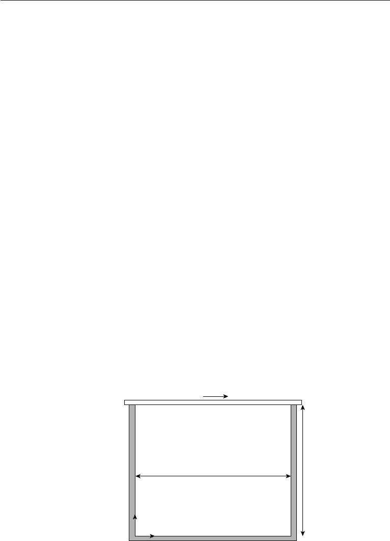
The driven cavity ﬂow problem, in which a ﬂuid-ﬁlled square box (“cavity”) is swirled

by a uniformly translating lid as shown in Figure 11.6, is a classic problem in CFD.

This problem is unambiguous with easily applied boundary conditions and has a

wealth of documented analytical and computational results, for example Ghia et al.

(1982). We will solve this ﬂow using the explicit MacCormack scheme discussed in

the previous section.

We may nondimensionalize the problem with the following scaling: lengths with

D, velocity with U, time with D

U, density with a reference density ρ

, and pressure

with ρ

. Using this scaling, the equation of state (11.99) becomes p = ρ

where M = U

c is the Mach number. The Reynolds number is deﬁned as Re =

µ.

The boundary conditions for this problem are relatively simple. The velocity

components on all four sides of the cavity are well deﬁned. There are two singularities

of velocity gradient at the two top corners where velocity u drops from U to 0 directly

underneath the sliding lid. However, these singularities will be smoothed out on a given

grid, since the change of the velocity occurs linearly between two grid points. The

boundary conditions for the density (hence the pressure) are more involved. Since the

density is not speciﬁed on a solid surface, we need to generate an update scheme for

Figure 11.6 Driven cavity ﬂow problem. The cavity is ﬁlled with a ﬂuid with the top lid sliding at a

constant velocity U.

5. Three Examples 441

values of density on all boundary points. A natural option is to derive that using the

continuity equation.

Consider the boundary on the left (at x = 0). Since v = 0 along the surface, the

continuity equation (11.96) reduces to

∂ρ

∂t

∂ρu

∂x

= 0. (11.138)

We may use a predictor-corrector scheme to update density on this surface with

a one-sided second-order accurate discretization for the spatial derivative,



∂f

∂x



2x

(

−f

i+2

+ 4f

i+1

− 3f

)

+ O



x





∂f

∂x



−1

2x

(

−f

i−2

+ 4f

i−1

− 3f

)

+ O



x



Therefore, on the surface of x = 0 (for i = 0 including two corner points on the left),

we have the following update scheme for density,

predictor ρ

∗

i,j

= ρ

i,j

−

t

2x



−

(

ρu

)

i+2,j

+ 4

(

ρu

)

i+1,j

− 3

(

ρu

)

i,j



(11.139)

corrector 2ρ

n+1

i,j

= ρ

i,j

+ ρ

∗

i,j

−

t

2x



−

(

ρu

)

∗

i+2,j

+ 4

(

ρu

)

∗

i+1,j

− 3

(

ρu

)

∗

i,j



(11.140)

Similarly, on the right side of the cavity x = D (for i = n

− 1, where n

is the

number of grid points in the x-direction, including two corner points on the right),

we have

predictor ρ

∗

i,j

= ρ

i,j

t

2x



−

(

ρu

)

i−2,j

+ 4

(

ρu

)

i−1,j

− 3

(

ρu

)

i,j



(11.141)

corrector 2ρ

n+1

i,j

= ρ

i,j

+ ρ

∗

i,j

t

2x



−

(

ρu

)

∗

i−2,j

+ 4

(

ρu

)

∗

i−1,j

− 3

(

ρu

)

∗

i,j



(11.142)

On the bottom of the cavity y = 0(j = 0),

predictor ρ

∗

i,j

= ρ

i,j

−

t

2y



−

(

ρv

)

i,j+2

+ 4

(

ρv

)

i,j+1

− 3

(

ρv

)

i,j



, (11.143)

corrector 2ρ

n+1

i,j

= ρ

i,j

+ ρ

∗

i,j

−

t

2y



−

(

ρv

)

∗

i,j+2

+ 4

(

ρv

)

∗

i,j+1

− 3

(

ρv

)

∗

i,j



(11.144)

Finally, on the top of the cavityy = D (j = n

− 1 where n

is the number of

grid points in the y-direction), the density needs to be updated from slightly different

expressions since ∂ρu

∂x = U∂ρ

∂x is not zero there,