Cohen I.M., Kundu P.K. Fluid Mechanics

Подождите немного. Документ загружается.

412 Computational Fluid Dynamics

During the past four decades different types of numerical methods have been

developed to simulate ﬂuid ﬂows involving a wide range of applications. These

methods include ﬁnite difference, ﬁnite element, ﬁnite volume, and spectral methods.

Some of them will be discussed in this chapter.

The CFD predictions are never completely exact. Because many sources of error

are involved in the predictions, one has to be very careful in interpreting the results

produced by CFD techniques. The most common sources of error are:

• Discretization error. This is intrinsic to all numerical methods. This error is

incurred whenever a continuous system is approximated by a discrete one where

a ﬁnite number of locations in space (grids) or instants of time may have been

used to resolve the ﬂow ﬁeld. Different numerical schemes may have different

orders of magnitude of the discretization error. Even with the same method,

the discretization error will be different depending upon the distribution of the

grids used in a simulation. In most applications, one needs to properly select a

numerical method and choose a grid to control this error to an acceptable level.

• Input data error. This is due to the fact that both ﬂow geometry and ﬂuid

properties may be known only in an approximate way.

• Initial and boundary condition error. It is common that the initial and boundary

conditions of a ﬂow ﬁeld may represent the real situation too crudely. For

example, ﬂow information is needed at locations where ﬂuid enters and leaves

the ﬂow geometry. Flow properties generally are not known exactly and are

thus only approximated.

• Modeling error. More complicated ﬂows may involve physical phenomena that

are not perfectly described by current scientiﬁc theories. Models used to solve

these problems certainly contain errors, for example, turbulence modeling,

atmospheric modeling, problems in multiphase ﬂows, and so on.

As a research and design tool, CFD normally complements experimental and

theoretical ﬂuid dynamics. However, CFD has a number of distinct advantages:

• It can be produced inexpensively and quickly. Although the price of most items

is increasing, computing costs are falling. According to Moore’s law based on

the observation of the data for the last 40 years, the CPU power will double

every 18 months into the foreseeable future.

• It generates complete information. CFD produces detailed and comprehensive

information of all relevant variables throughout the domain of interest. This

information can also be easily accessed.

• It allows easy change of the parameters. CFD permits input parameters to be

varied easily over wide ranges, thereby facilitating design optimization.

• It has the ability to simulate realistic conditions. CFD can simulate ﬂows directly

under practical conditions, unlike experiments, where a small- or a large-scale

model may be needed.

2. Finite Difference Method 413

• It has the ability to simulate ideal conditions. CFD provides the convenience

of switching off certain terms in the governing equations, which allows one

to focus attention on a few essential parameters and eliminate all irrelevant

features.

• It permits exploration of unnatural events. CFD allows events to be studied that

every attempt is made to prevent, for example, conﬂagrations, explosions, or

nuclear power plant failures.

2. Finite Difference Method

The key to various numerical methods is to convert the partial different equations

that govern a physical phenomenon into a system of algebraic equations. Different

techniques are available for this conversion. The ﬁnite difference method is one of

the most commonly used.

Approximation to Derivatives

Consider the one-dimensional transport equation,

∂T

∂t

+ u

∂T

∂x

= D

∂

∂x

for 0  x  L. (11.1)

This is the classic convection-diffusion problem for T(x,t), where u is a convective

velocity and D is a diffusion coefﬁcient. For simplicity, let us assume that u and D

are two constants. This equation is written in nondimensional form. The boundary

conditions for this problem are

(

0,t

)

= g and

∂T

∂x

(

L, t

)

= q, (11.2)

where g and q are two constants. The initial condition is

(

x,0

)

= T

(

)

for 0  x  L, (11.3)

where T

(

)

is a given function that satisﬁes the boundary conditions (11.2).

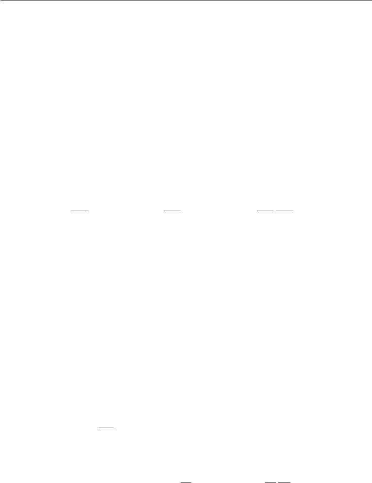
Let us ﬁrst discretize the transport equation (11.1) on a uniform grid with a grid

spacing x, as shown in Figure 11.1. Equation (11.1) is evaluated at spatial location

x = x

and time t = t

. Deﬁne T

(

)

as the exact value of T at the location x = x

and time t = t

, and let T

be its approximation. Using the Taylor series expansion,

we have

i+1

+x



∂T

∂x



x



∂

∂x



x



∂

∂x



x



∂

∂x





x



(11.4)

i−1

−x



∂T

∂x



x



∂

∂x



−

x



∂

∂x



x



∂

∂x





x



(11.5)

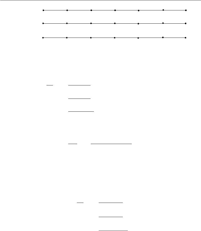
414 Computational Fluid Dynamics

n+1

n21

∆ x ∆ x

i21

i+1

50 x

Figure 11.1 Uniform grid in space and time.

where O



x



means terms of the order of x

. Therefore, the ﬁrst spatial derivative

may be approximated as



∂T

∂x



i+1

− T

x

+ O

(

x

)

(forward difference)

− T

i−1

x

+ O

(

x

)

(backward difference)

i+1

− T

i−1

2x

+ O



x



(centered difference)

(11.6)

and the second order derivative may be approximated as



∂

∂x



i+1

− 2T

+ T

i−1

x

+ O



x



. (11.7)

The orders of accuracy of the approximations (truncation errors) are also indicated in

the expressions of (11.6) and (11.7). More accurate approximations generally require

more values of the variable on the neighboring grid points. Similar expressions can

be derived for nonuniform grids.

In the same fashion, the time derivative can be discretized as



∂T

∂t



n+1

− T

t

+ O

(

t

)

− T

n−1

t

+ O

(

t

)

n+1

− T

n−1

2t

+ O



t



(11.8)

where t = t

n+1

− t

= t

− t

n−1

is the constant time step.

Discretization and Its Accuracy

A discretization of the transport equation (11.1) is obtained by evaluating the equa-

tion at ﬁxed spatial and temporal grid points and using the approximations for the

individual derivative terms listed in the preceding section. When the ﬁrst expression

in (11.8) is used, together with (11.7) and the centered difference in (11.6), (11.1)

2. Finite Difference Method 415

may be discretized by

n+1

− T

t

+ u

i+1

− T

i−1

2x

= D

i+1

− 2T

+ T

i−1

x

+ O



t, x



, (11.9)

n+1

≈ T

− ut

i+1

− T

i−1

2x

+ Dt

i+1

− 2T

+ T

i−1

x

(11.10)

= T

− α



i+1

− T

i−1



+ β



i+1

− 2T

+ T

i−1



where

α = u

t

2x

,β= D

t

x

. (11.11)

Once the values of T

are known, starting with the initial condition (11.3), the expres-

sion (11.10) simply updates the variable for the next time step t = t

n+1

. This scheme

is known as an explicit algorithm. The discretization (11.10) is ﬁrst order accurate in

time and second order accurate in space.

As another example, when the backward difference expression in (11.8) is used,

we will have

− T

n−1

t

+ u

i+1

− T

i−1

2x

= D

i+1

− 2T

+ T

i−1

x

+ O



t, x



, (11.12)

+ α



i+1

− T

i−1



− β



i+1

− 2T

+ T

i−1



≈ T

n−1

. (11.13)

At each time step t = t

, here a system of algebraic equations needs to be solved to

advance the solution. This scheme is known as an implicit algorithm. Obviously, for

the same accuracy, the explicit scheme (11.10) is much simpler than the implicit one

(11.13). However, the explicit scheme has limitations.

Convergence, Consistency, and Stability

The result from the solution of the explicit scheme (11.10) or the implicit scheme

(11.13) represents an approximate numerical solution to the original partial differen-

tial equation (11.1). One certainly hopes that the approximate solution will be close

to the exact one. Thus we introduce the concepts of convergence, consistency, and

stability of the numerical solution.

The approximate solution is said to be convergent if it approaches the exact

solution as the grid spacings x and t tend to zero. We may deﬁne the solution

error as the difference between the approximate solution and the exact solution,

= T

− T

(

)

. (11.14)

416 Computational Fluid Dynamics

Thus the approximate solution converges when e

→ 0asx, t → 0. For a

convergent solution, some measure of the solution error can be estimated as



 Kx

t

, (11.15)

where the measure may be the root mean square (rms) of the solution error on all the

grid points; K is a constant independent of the grid spacing x and the time step

t; the indices a and b represent the convergence rates at which the solution error

approaches zero.

One may reverse the discretization process, and examine the limit of the dis-

cretized equations (11.10) and (11.13), as the grid spacing tends to zero. The dis-

cretized equation is said to be consistent if it recovers the original partial differential

equation (11.1) in the limit of zero grid spacing.

Let us consider the explicit scheme (11.10). Substitution of the Taylor series

expansions (11.4) and (11.5) into this scheme (11.10) produces,



∂T

∂t



+ u



∂T

∂x



− D



∂

∂x



+ E

= 0, (11.16)

where

t



∂

∂t



x



∂

∂x



−D

x



∂

∂x





t

,x



, (11.17)

is the truncation error. Obviously, as the grid spacing x, t → 0, this truncation

error is of the order of O



t, x



and tends to zero. Therefore, the explicit scheme

(11.10) or expression (11.16) recovers the original partial differential equation (11.1),

or it is consistent. It is said to be ﬁrst-order accurate in time and second-order accurate

in space, according to the order of magnitude of the truncation error.

In addition to the truncation error introduced in the discretization process, other

sources of error may be present in the approximate solution. Spontaneous disturbances

(such as the round-off error) may be introduced during either the evaluation or the

numerical solution process. A numerical approximation is said to be stable if these

disturbances decay and do not affect the solution.

The stability of the explicit scheme (11.10) may be examined using the von

Neumann method. Let us consider the error at a grid point,

= T

− T

, (11.18)

where T

is the exact solution of the discretized system (11.10) and T

is the approxi-

mate numerical solution of the same system. This error could be introduced due to the

round-off error at each step of the computation. We need to monitor its decay/growth

with time. It can be shown that the evolution of this error satisﬁes the same homoge-

neous algebraic system (11.10) or

n+1

(

α + β

)

i−1

(

1 − 2β

)

(

β − α

)

i+1

. (11.19)

2. Finite Difference Method 417

The error distributed along the grid line can always be decomposed in Fourier

space as

∞



k=−∞

(

)

iπkx

(11.20)

where i =

√

−1, k is the wavenumber in Fourier space, and g

represents the function

g at time t = t

. As the system is linear, we can examine one component of (11.20)

at a time,

= g

(k)e

iπkx

. (11.21)

The component at the next time level has a similar form

n+1

= g

n+1

(k)e

iπkx

. (11.22)

Substituting the preceding two equations (11.21) and (11.22) into error equation

(11.19), we obtain,

n+1

iπkx

= g

[(α + β)e

iπkx

i−1

+ (1 − 2β)e

iπkx

+ (β −α)e

iπkx

i+1

] (11.23)

n+1

=[(α + β)e

−iπkx

+ (1 − 2β) +(β − α)e

iπkx

]. (11.24)

This ratio g

n+1

is called the ampliﬁcation factor. The condition for stability is that

the magnitude of the error should decay with time, or



n+1



 1, (11.25)

for any value of the wavenumber k. For this explicit scheme, the condition for stability

(11.25) can be expressed as



1 − 4β sin





(

2α sin θ

)

 1, (11.26)

where θ = kπx. The stability condition (11.26) also can be expressed as (Noye,

1983),

0  4α

 2β  1. (11.27)

For the pure diffusion problem (u = 0), the stability condition (11.27) for this

explicit scheme requires that

0  β 

or t 

x

, (11.28)

which limits the size of the time step. For the pure convection problem (D = 0),

condition (11.27) will never be satisﬁed, which indicates that the scheme is always

418 Computational Fluid Dynamics

unstable and it means that any error introduced during the computation will explode

with time. Thus, this explicit scheme is useless for pure convection problems. To

improve the stability of the explicit scheme for the convection problem, one may use

an upwind scheme to approximate the convective term,

n+1

= T

− 2α



− T

i−1



, (11.29)

where the stability condition requires that

t

x

 1. (11.30)

The condition (11.30) is known as the Courant-Friedrichs-Lewy (CFL) condition.

This condition indicates that a ﬂuid particle should not travel more than one spatial

grid in one time step.

It can easily be shown that the implicit scheme (11.13) is also consistent and

unconditionally stable.

It is normally difﬁcult to show the convergence of an approximate solution theo-

retically. However, the Lax Equivalence Theorem (Richtmyer and Morton, 1967)

states that: for an approximation to a well-posed linear initial value problem, which

satisﬁes the consistency condition, stability is a necessary and sufﬁcient condition for

the convergence of the solution.

For convection-diffusion problems, the exact solution may change signiﬁcantly

in a narrow boundary layer. If the computational grid is not sufﬁciently ﬁne to resolve

the rapid variation of the solution in the boundary layer, the numerical solution may

present unphysical oscillations adjacent to or in the boundary layer. To prevent the

oscillatory solution, a condition on the cell Pecl

et number (or Reynolds number) is

normally required (see Section 4),

cell

= u

x

 2. (11.31)

3. Finite Element Method

The ﬁnite element method was developed initially as an engineering procedure for

stress and displacement calculations in structural analysis. The method was subse-

quently placed on a sound mathematical foundation with a variational interpretation

of the potential energy of the system. For most ﬂuid dynamics problems, ﬁnite ele-

ment applications have used the Galerkin ﬁnite element formulation on which we will

focus in this section.

Weak or Variational Form of Partial Differential Equations

Let us consider again the one-dimensional transport problem (11.1). The form of

(11.1) with the boundary condition (11.2) and the initial conditions (11.3) is called

the strong (or classical) form of the problem.

We ﬁrst deﬁne a collection of trial solutions, which consists of all functions

that have square-integrable ﬁrst derivatives (H

functions, i.e.



(

)

dx < ∞ if

3. Finite Element Method 419

T ∈ H

) and satisfy the Dirichlet type of boundary condition (where the value of the

variable is speciﬁed) at x = 0. This is expressed as the trial functional space,

S =





T ∈ H

(

)

= g



. (11.32)

The variational space of the trial solution is deﬁned as

V =





w ∈ H

(

)

= 0



, (11.33)

which requires a corresponding homogeneous boundary condition.

We next multiply the transport equation (11.1) by a function in the variational space

(w ∈ V), and integrate the product over the domain where the problem is deﬁned,





∂T

∂t



dx + u





∂T

∂x



dx = D





∂

∂x



dx. (11.34)

Integrating the right-hand-side of (11.34) by parts, we have





∂T

∂t



dx + u





∂T

∂x



dx + D





∂T

∂x

∂w

∂x



dx = D



∂T

∂x



= Dqw

(

)

, (11.35)

where the boundary conditions ∂T/∂x = q and w

(

)

= 0 are applied. The integral

equation (11.35) is called the weak form of this problem. Therefore, the weak form

can be stated as: Find T ∈ S such that for all w ∈ V ,





∂T

∂t



dx + u





∂T

∂x



dx + D





∂T

∂x

∂w

∂x



dx = Dqw

(

)

(11.36)

It can be formally shown that the solution of the weak problem is identical to that

of the strong problem, or that the strong and weak forms of the problem are equivalent.

Obviously, if T is a solution of the strong problem (11.1) and (11.2), it must also be a

solution of the weak problem (11.36) using the procedure for derivation of the weak

formulation. However, let us assume that T is a solution of the weak problem (11.36).

By reversing the order in deriving the weak formulation, we have





∂T

∂t

+ u

∂T

∂x

− D

∂

∂x



wdx + D



∂T

∂x

(

)

− q



(

)

= 0. (11.37)

Satisfying (11.37) for all possible functions of w ∈ V requires that

∂T

∂t

+ u

∂T

∂x

− D

∂

∂x

= 0 for x ∈

(

0,L

)

, and

∂T

∂x

(

)

− q = 0, (11.38)

420 Computational Fluid Dynamics

which means that this solution T will be also a solution of the strong problem. It

should be noted that the Dirichlet type of boundary condition (where the value of

the variable is speciﬁed) is built into the trial functional space S, and is thus called

an essential boundary condition. However, the Neumann type of boundary condition

(where the derivative of the variable is imposed) is implied by the weak formulation

as indicated in (11.38) and is referred to as a natural boundary condition.

Galerkin’s Approximation and Finite Element Interpolations

As we have shown, the strong and weak forms of the problem are equivalent, and there

is no approximation involved between these two formulations. Finite element methods

start with the weak formulation of the problem. Let us construct ﬁnite-dimensional

approximations of S and V , which are denoted by S

and V

, respectively. The super-

script refers to a discretization with a characteristic grid size h. The weak formulation

(11.36) can be rewritten using these new spaces, as: Find T

∈ S

such that for all

∈ V





∂T

∂t



dx + u





∂T

∂x



dx+D





∂T

∂x

∂w

∂x



dx = Dqw

(

)

(11.39)

Normally, S

and V

will be subsets of S and V , respectively. This means that if a

function φ ∈ S

then φ ∈ S, and if another function ψ ∈ V

then ψ ∈ V . Therefore,

(11.39) deﬁnes an approximate solution T

to the exact weak form of the problem

(11.36).

It should be noted that, up to the boundary condition T

(

)

= g, the function

spaces S

and V

are composed of identical collections of functions. We may take

out this boundary condition by deﬁning a new function

(

x,t

)

= T

(

x,t

)

− g

(

)

, (11.40)

where g

is a speciﬁc function that satisﬁes the boundary condition g

(

)

= g.

Thus, the functions v

and w

belong to the same space V

. Equation (11.39) can be

rewritten in terms of the new function v

: Find T

= v

, where v

∈ V

, such

that for all w

∈ V





∂v

∂t



dx + a





= Dqw

(

)

− a





. (11.41)

The operator a

(

·, ·

)

is deﬁned as

(

w, v

)

= u





∂v

∂x



dx + D





∂v

∂x

∂w

∂x



dx. (11.42)

The formulation (11.41) is called a Galerkin formulation, because the solution

and the variational functions are in the same space. Again, the Galerkin formulation

of the problem is an approximation to the weak formulation (11.36). Other classes

3. Finite Element Method 421

of approximation methods, called Petrov-Galerkin methods, are those in which the

solution function may be contained in a collection of functions other than V

Next we need to explicitly construct the ﬁnite-dimensional variational space

. Let us assume that the dimension of the space is n and that the basis (shape or

interpolation) functions for the space are

(

)

,A= 1, 2, ..., n. (11.43)

Each shape function has to satisfy the boundary condition at x = 0,

(

)

= 0,A= 1, 2, ..., n, (11.44)

which is required by the space V

. The form of the shape functions will be discussed

later. Any function w

∈ V

can be expressed as a linear combination of these shape

functions,



A=1

(

)

, (11.45)

where the coefﬁcients c

are independent of x and uniquely deﬁne this function. We

may introduce one additional function N

to specify the function g

in (11.40) related

to the essential boundary condition. This shape function has the property

(

)

= 1. (11.46)

Therefore, the function g

can be expressed as

(

)

= gN

(

)

, and g

(

)

= g. (11.47)

With these deﬁnitions, the approximate solution can be written as

(

x,t

)



A=1

(

)

(

)

, (11.48)

and

(

x,t

)



A=1

(

)

(

)

+ gN

(

)

, (11.49)

where d

’s are functions of time only for time dependent problems.

Matrix Equations, Comparison with Finite Difference Method

With the construction of the ﬁnite-dimensional space V

, the Galerkin formulation

of the problem (11.41) leads to a coupled system of ordinary differential equations.