Cohen I.M., Kundu P.K. Fluid Mechanics

Подождите немного. Документ загружается.

392 Boundary Layers and Related Topics

An asymptotic expansion is a ﬁnite sequence of limit statements of the type

written in the preceding. For example, because lim

ε→0

(sin ε)/ε = 1, sin ε = ε+o(ε).

Following up using the powers of ε as gauge functions,

lim

ε→0

(sin ε − ε)/ε

=−

, sin ε = ε −

+ o(

By continuing this process we can establish that the term o(ε

) is better represented

by O(ε

) and is in fact 

/5!. The series terminates with the order symbol.

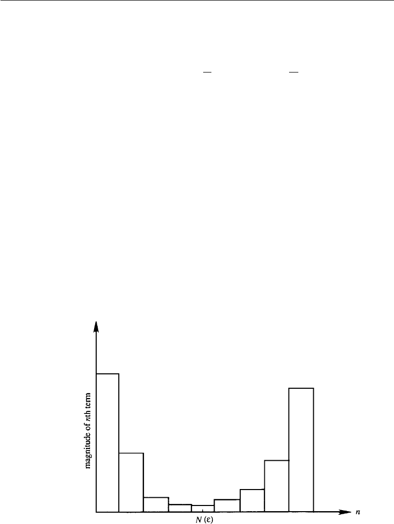
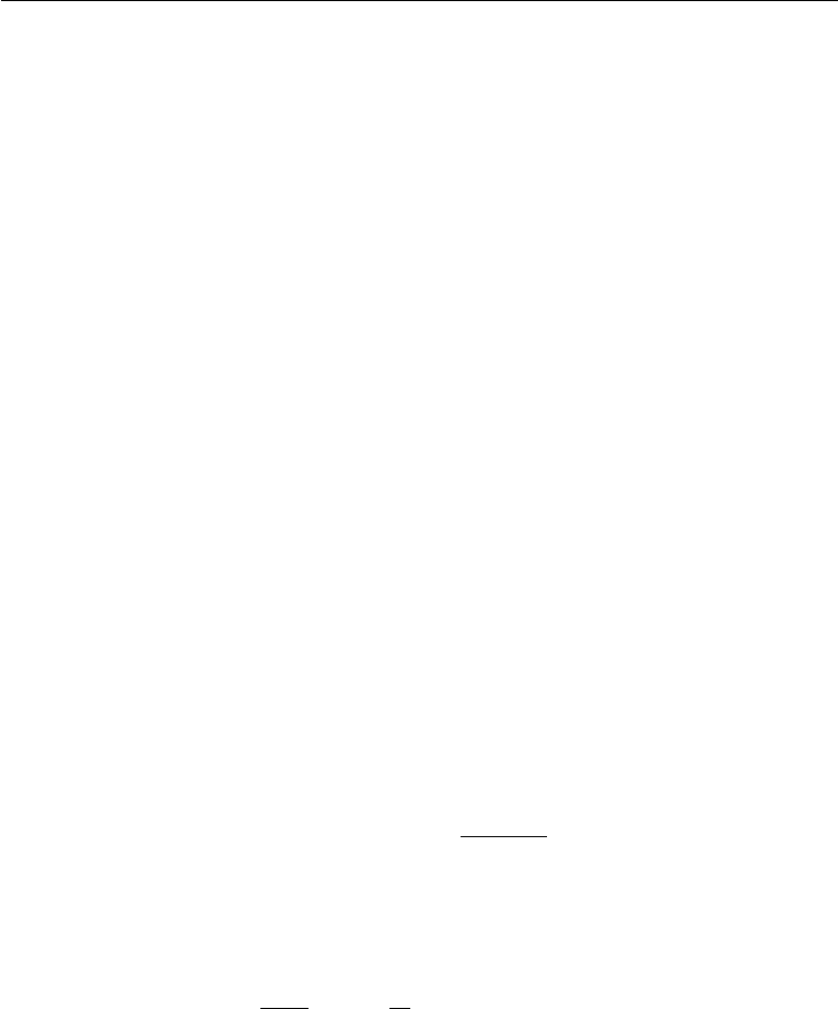
The interesting property of an asymptotic expansion is that the series (10.58) may

not converge if extended indeﬁnitely. Thus, for a ﬁxed ε, the magnitude of a term may

eventually increase as shown in Figure 10.32. Therefore, there is an optimum number

of terms N(ε) at which the series should be truncated. The number N(ε) is difﬁcult

to guess, but that is of little consequence, because only one or two terms in the

asymptotic expansion are calculated. The accuracy of the asymptotic representation

can be arbitrarily improved by keeping n ﬁxed, and letting ε → 0.

We here emphasize the distinction between convergence and asymptoticity. In

convergence we are concerned with terms far out in an inﬁnite series, a

. We must

have lim

n→∞

= 0 and, for example, lim

n→∞

n+1

| < 1 for convergence.

Asymptoticity is a different limit: n is ﬁxed at a ﬁnite number and the approximation

is improved as ε (say) tends to its limit.

Figure 10.32 Terms in a divergent asymptotic series, in which N(ε) indicates the optimum number of

terms at which the series should be truncated. M. Van Dyke, Perturbation Methods in Fluid Mechanics,

1975 and reprinted with the permission of Prof. Milton Van Dyke for The Parabolic Press.

14. Perturbation Techniques 393

The value of an asymptotic expansion becomes clear if we compare the

convergent series for a Bessel function J

(x), given by

(x) = 1 −

−

+···, (10.59)

with the ﬁrst term of its asymptotic expansion

(x) ∼



πx

cos



x −



as x →∞. (10.60)

The convergent series (10.59) is useful when x is small, but more than eight terms

are needed for three-place accuracy when x exceeds 4. In contrast, the one-term

asymptotic representation (10.60) gives three-place accuracy for x>4. Moreover,

the asymptotic expansion indicates the shape of the function, whereas the inﬁnite

series does not.

Nonuniform Expansion

In many situations we develop an asymptotic expansion for a function of two

variables, say

f(x; ε) ∼



(x)g

(ε) as ε → 0. (10.61)

If the expansion holds for all values of x, it is called uniformly valid in x, and the prob-

lem is described as a regular perturbation problem. In this case any successive term

is smaller than the preceding term for all x. In some interesting situations, however,

the expansion may break down for certain values of x. For such values of x, a

(x)

increases faster with m than g

(ε) decreases with m, so that the term a

(x)g

(ε) is

not smaller than the preceding term. When the asymptotic expansion (10.61) breaks

down for certain values of x, it is called a nonuniform expansion, and the problem is

called a singular perturbation problem. For example, the series

1 + εx

= 1 −εx + ε

− ε

+···, (10.62)

is nonuniformly valid, because it breaks down when εx = O(1). No matter how small

we make ε, the second term is not a correction of the ﬁrst term for x>1/ε.Wesay

that the singularity of the perturbation expansion (10.62) is at large x or at inﬁnity.

On the other hand, the expansion

√

x + ε =

√



1 +



1/2

√



1 +

−

+···



, (10.63)

is nonuniform because it breaks down when ε/x = O(1). The singularity of this

expansion is at x = 0, because it is not valid for x<ε. The regions of nonuniformity

are called boundary layers; for equation (10.62) it is x>1/ε, and for equation (10.63)

394 Boundary Layers and Related Topics

it is x<ε. To obtain expansions that are valid within these singular regions, we need

to write the solution in terms of a variable η which is of order 1 within the region

of nonuniformity. It is evident that η = εx for equation (10.62), and η = x/ε for

equation (10.63).

In many cases, singular perturbation problems are associated with the small

parameter ε multiplying the highest order derivative (as in viscous boundary layer

problems), so that the differential equation drops by one order as ε → 0, resulting in

an inability to satisfy all the boundary conditions. In several other singular perturbation

problems the small parameter does not multiply the highest-order derivative. An

example is low Reynolds number ﬂows, for which the nondimensional governing

equation is

εu ·∇u =−∇p +∇

where ε = Re  1. In this case the singularity or nonuniformity is at inﬁnity. This is

discussed in Section 9.13.

15. An Example of a Regular Perturbation Problem

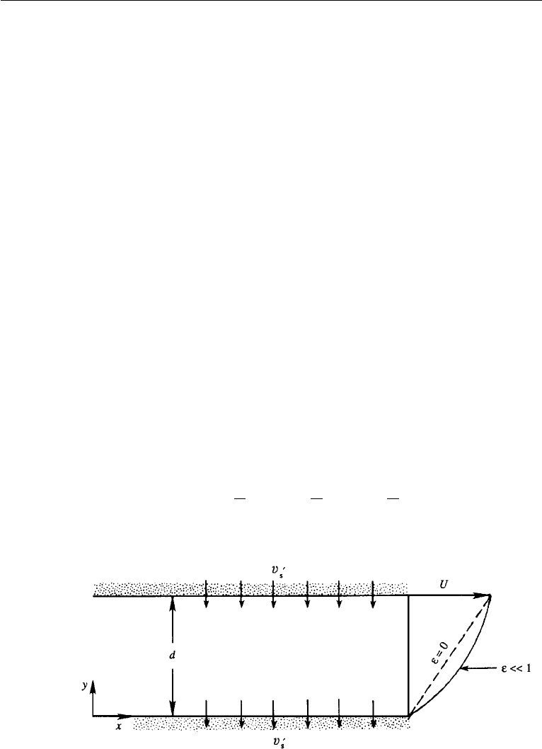
As a simple example of a perturbation expansion that is uniformly valid everywhere,

consider a plane Couette ﬂow with a uniform suction across the ﬂow (Figure 10.33).

The upper plate is moving parallel to itself at speed U and the lower plate is station-

ary. The distance between the plates is d and there is a uniform downward suction

velocity v



, with the ﬂuid coming in through the upper plate and going out through the

bottom. For notational simplicity, we shall denote dimensional variables by a prime

and nondimensional variables without primes:

y =



,u=



,v=



Figure 10.33 Uniform suction in a Couette ﬂow, showing the velocity proﬁle u(y) for ε = 0 and ε  1.

15. An Example of a Regular Perturbation Problem 395

As ∂/∂x = 0 for all variables, the nondimensional equations are

∂v

∂y

= 0 (continuity), (10.64)

(x-momentum), (10.65)

subject to

v(0) = v(1) =−v

, (10.66)

u(0) = 0, (10.67)

u(1) = 1, (10.68)

where Re = Ud/ν, and v

= v



/U.

The continuity equation shows that the lateral ﬂow is independent of y and

therefore must be

v(y) =−v

to satisfy the boundary conditions on v. The x-momentum equation then becomes

+ ε

= 0, (10.69)

where ε = v

Re = v



d/ν. We assume that the suction velocity is small, so that ε  1.

The problem is to solve equation (10.69), subject to equations (10.67) and (10.68).

An exact solution can easily be found for this problem, and will be presented at the

end of this section. However, an exact solution may not exist in more complicated

problems, and we shall illustrate the perturbation approach. We try a perturbation

solution in integral powers of ε, of the form,

u(y) = u

(y) + εu

(y) + ε

(y) + O(ε

). (10.70)

(A power series in ε may not always be possible, as remarked upon in the preceding

section.) Our task is to determine u

(y), u

(y), etc.

Substituting equation (10.70) into equations (10.69), (10.67), and (10.68), we

obtain

+ ε





+ ε





+ O(ε

) = 0, (10.71)

subject to

(0) + εu

(0) + ε

(0) + O(ε

) = 0, (10.72)

(1) + εu

(1) + ε

(1) + O(ε

) = 1. (10.73)

396 Boundary Layers and Related Topics

Equations for the various orders are obtained by taking the limits of equations

(10.71)–(10.73) as ε → 0, then dividing by ε and taking the limit ε → 0 again,

and so on. This is equivalent to equating terms with like powers of ε. Up to order ε,

this gives the following sets:

Order ε

= 0,

(0) = 0,u

(1) = 1.

(10.74)

Order ε

=−

(0) = 0,u

(1) = 0.

(10.75)

The solution of the zero-order problem (10.74) is

= y. (10.76)

Substituting this into the ﬁrst-order problem (10.75), we obtain the solution

(1 − y).

The complete solution up to order ε is then

u(y) = y +

[y(1 −y)]+O(ε

). (10.77)

In this expansion the second term is less than the ﬁrst term for all values of y as ε → 0.

The expansion is therefore uniformly valid for all y and the perturbation problem is

regular. A sketch of the velocity proﬁle (10.77) is shown in Figure 10.33.

It is of interest to compare the perturbation solution (10.77) with the exact solu-

tion. The exact solution of (10.69), subject to equations (10.67) and (10.68), is easily

found to be

u(y) =

1 − e

−εy

1 − e

−ε

. (10.78)

For ε  1, Equation (10.78) can be expanded in a power series of ε, where the ﬁrst

few terms are identical to those in equation (10.77).

16. An Example of a Singular Perturbation Problem

Consider again the problem of uniform suction across a plane Couette ﬂow, discussed

in the preceding section. For the case of weak suction, namely ε = v



d/ν  1, we

saw that the perturbation problem is regular and the series is uniformly valid for all

16. An Example of a Singular Perturbation Problem 397

values of y. A more interesting case is that of strong suction, deﬁned as ε  1, for

which we shall now see that the perturbation expansion breaks down near one of the

walls. As before, the v-ﬁeld is uniform everywhere:

v(y) =−v

The governing equation is (10.69), which we shall now write as

= 0, (10.79)

subject to

u(0) = 0, (10.80)

u(1) = 1, (10.81)

where we have deﬁned

δ ≡



 1,

as the small parameter. We try an expansion in powers of δ:

u(y) = u

(y) + δu

(y) + δ

(y) + O(δ

). (10.82)

Substitution into equation (10.79) leads to

= 0. (10.83)

The solution of this equation is u

= const., which cannot satisfy conditions at both

y = 0 and y = 1. This is expected, because as δ → 0 the highest order derivative

drops out of the governing equation (10.79), and the approximate solution cannot

satisfy all the boundary conditions. This happens no matter how many terms are

included in the perturbation series. A boundary layer is therefore expected near one

of the walls, where the solution varies so rapidly that the two terms in equation (10.79)

are of the same order.

The expansion (10.82), valid outside the boundary layers, is the “outer” expan-

sion, the ﬁrst term of which is governed by equation (10.83). If the outer expansion

satisﬁes the boundary condition (10.80), then the ﬁrst term in the expansion is u

= 0;

if on the other hand the outer expansion satisﬁes the condition (10.81), then u

= 1.

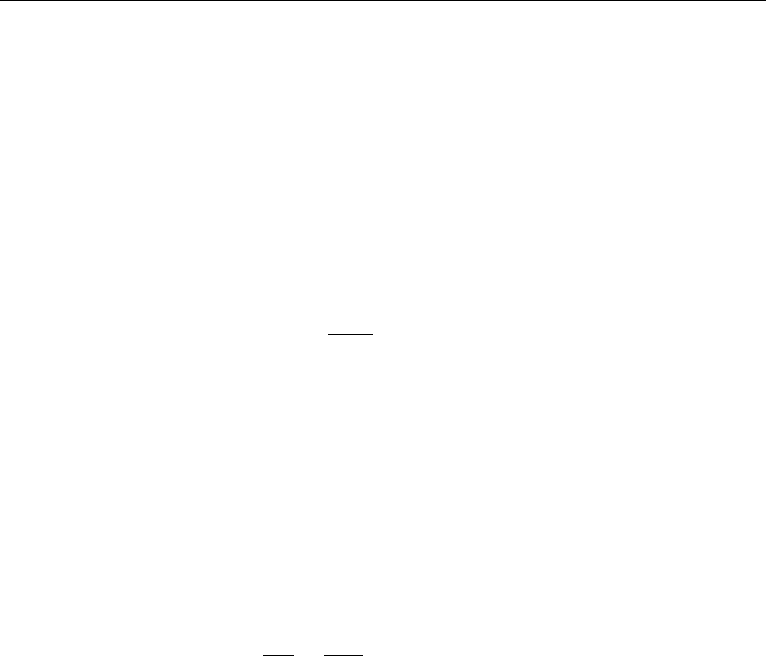
The outer expansion should be smoothly matched to an “inner” expansion valid within

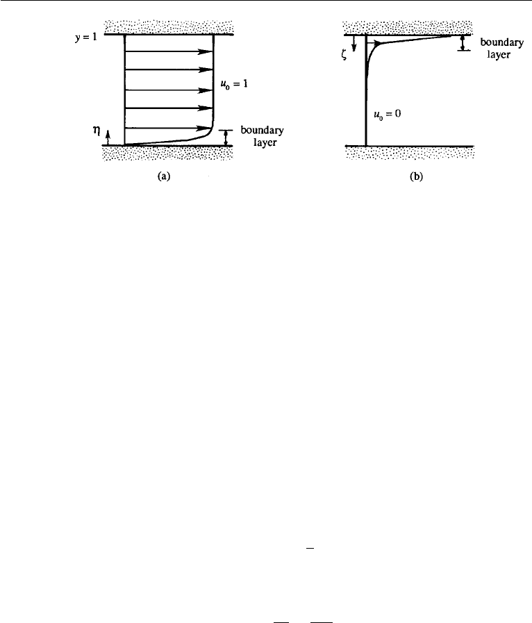
the boundary layer. The two possibilities are sketched in Figure 10.34, where it is

evident that a boundary layer occurs at the top plate if u

= 0, and it occurs at the

bottom plate if u

= 1. Physical reasons suggest that a strong suction would tend

to keep the proﬁle of the longitudinal velocity uniform near the wall through which

the ﬂuid enters, so that a boundary layer at the lower wall seems more reasonable.

Moreover, the ε  1 case is then a continuation of the ε  1 behavior (Figure 10.33).

398 Boundary Layers and Related Topics

Figure 10.34 Couette ﬂow with strong suction, showing two possible locations of the boundary layer.

The one shown in (a) is the correct one.

We shall therefore proceed with this assumption and verify later in the section that it

is not mathematically possible to have a boundary layer at y = 1.

The location of the boundary layer is determined by the sign of the ratio of the

dominant terms in the boundary layer. This is the case because the boundary layer

must always decay into the domain and the decay is generally exponential. The inward

decay is required so as to match with the outer region solution. Thus a ratio of signs

that is positive (when both terms are on the same side of the equation) requires the

boundary layer to be at the left or bottom, that is, the boundary with the smaller

coordinate.

The ﬁrst task is to determine the natural distance within the boundary layer, where

both terms in equation (10.79) must be of the same order. If y is a typical distance

within the boundary layer, this requires that δ/y

= O(1/y), that is

y = O(δ),

showing that the natural scale for measuring distances within the boundary layer is δ.

We therefore deﬁne a boundary layer coordinate

η ≡

which transforms the governing equation (10.79) to

−

dη

. (10.84)

As in the Blasius solution, η = O(1) within the boundary layer and η →∞far

outside of it.

The solution of equation (10.84) as η →∞is to be matched to the solution of

equation (10.79) as y → 0. Another way to solve the problem is to write a composite

expansion consisting of both the outer and the inner solutions:

u(y) =[u

(y) + δu

(y) +···]+{ˆu

(η) + δ ˆu

(η) +···}, (10.85)

16. An Example of a Singular Perturbation Problem 399

where the term within {}is regarded as the correction to the outer solution within

the boundary layer. All terms in the boundary layer correction {}go to zero as

η →∞. Substituting equation (10.85) into equation (10.79), we obtain

+ δ





+ δ



+ O(δ

)

+ δ

−1



d ˆu

dη

ˆu

dη





d ˆu

dη

ˆu

dη



+ O(δ) = 0. (10.86)

A systematic procedure is to multiply equation (10.86) by powers of δ and take limits

as δ → 0, with ﬁrst y held ﬁxed and then η held ﬁxed. When y is held ﬁxed (which

we write as y = O(1)) and δ → 0, the boundary layer becomes progressively thinner

and we move outside and into the outer region. When η is held ﬁxed (i.e, η = O(1))

and δ → 0, we obtain the behavior within the boundary layer.

Multiplying equation (10.86) by δ and taking the limit as δ → 0, with η = O(1),

we obtain

d ˆu

dη

ˆu

dη

= 0, (10.87)

which governs the ﬁrst term of the boundary layer correction. Next, the limit of

equation (10.86) as δ → 0, with y = O(1),gives

= 0, (10.88)

which governs the ﬁrst term of the outer solution. (Note that in this limit η →∞,

and consequently we move outside the boundary layer where all correction terms

go to zero, that is d ˆu

/dη → 0 and d

ˆu

/dη

→ 0.) The next largest term

in equation (10.86) is obtained by considering the limit δ → 0 with η = O(1),

giving

d ˆu

dη

ˆu

dη

= 0,

and so on. It is clear that our formal limiting procedure is equivalent to setting the

coefﬁcients of like powers of δ in equation (10.86) to zero, with the boundary layer

terms treated separately.

As the composite expansion holds everywhere, all boundary conditions can be

applied on it. With the assumed solution of equation (10.85), the boundary condition

equations (10.80) and (10.81) give

(0) +ˆu

(0) + δ[u

(0) +ˆu

(0)]+···=0, (10.89)

(1) + 0 + δ[u

(1) + 0]+···=1. (10.90)

400 Boundary Layers and Related Topics

Equating like powers of δ, we obtain the following conditions

(0) +ˆu

(0) = 0,u

(0) +ˆu

(0) = 0, (10.91)

(1) = 1,u

(1) = 0. (10.92)

We can now solve equation (10.88) along with the ﬁrst condition in equation (10.92),

obtaining

(y) = 1. (10.93)

Next, we can solve equation (10.87), along with the ﬁrst condition in equation (10.91),

namely

ˆu

(0) =−u

(0) =−1,

and the condition ˆu

(∞) = 0. The solution is

ˆu

(η) =−e

−η

To the lowest order, the composite expansion is, therefore,

u(y) = 1 − e

−η

= 1 −e

−y/δ

, (10.94)

which we have written in terms of both the inner variable η and the outer vari-

able y, because the composite expansion is valid everywhere. The ﬁrst term is the

lowest-order outer solution, and the second term is the lowest-order correction in the

boundary layer.

Comparison with Exact Solution

The exact solution of the problem is (see equation (10.78)):

u(y) =

1 − e

−y/δ

1 − e

−1/δ

. (10.95)

We want to write the exact solution in powers of δ and compare with our perturbation

solution. An important result to remember is that exp (−1/δ) decays faster than any

power of δ as δ → 0, which follows from the fact that

lim

δ→0

−1/δ

= lim

ε→∞

= 0,e

−1/δ

= o(δ

), n > 0,

for any n, as can be veriﬁed by applying the l’Hˆopital rule n times. Thus, the denomi-

nator in equation (10.95) exponentially approaches 1, with no contribution in powers

of δ. It follows that the expansion of the exact solution in terms of a power series in

δ is

u(y)  1 − e

−y/δ

, (10.96)

17. Decay of a Laminar Shear Layer 401

which agrees with our composite expansion (10.94). Note that no terms in powers of

δ enter in equation (10.96). Although in equation (10.94) we did not try to continue

our series to terms of order δ and higher, the form of equation (10.96) shows that these

extra terms would have turned out to be zero if we had calculated them. However, the

nonexistence of terms proportional to δ and higher is special to the current problem,

and not a frequent event.

Why There Cannot Be a Boundary Layer at y = 1

So far we have assumed that the boundary layer could occur only at y = 0. Let us

now investigate what would happen if we assumed that the boundary layer happened

to be at y = 1. In this case we deﬁne a boundary layer coordinate

ζ ≡

1 − y

, (10.97)

which increases into the ﬂuid from the upper wall (Figure 10.34b). Then the

lowest-order terms in the boundary conditions (10.91) and (10.92) are replaced by

(0) = 0,

(1) +ˆu

(0) = 1,

where ˆu

(0) represents the value of ˆu

at the upper wall where ζ = 0. The ﬁrst

condition gives the lowest-order outer solution u

(y) = 0. To ﬁnd the lowest-order

boundary layer correction ˆu

(ζ ), note that the equation governing it (obtained by

substituting equation (10.97) into equation (10.87)) is

d ˆu

dζ

−

ˆu

dζ

= 0, (10.98)

subject to

ˆu

(0) = 1 − u

(1) = 1,

ˆu

(∞) = 0.

A substitution of the form ˆu

(ζ ) = exp(aζ ) into equation (10.103) shows that a =

+1, so that the solution to equation (10.98) is exponentially increasing in ζ and cannot

satisfy the condition at ζ =∞.

17. Decay of a Laminar Shear Layer

It is shown in Chapter 12 (pp. 515–516) that ﬂows exhibiting an inﬂection point

in the streamwise velocity proﬁle are highly unstable. These results, based on the

Orr-Sommerfeld analysis for parallel ﬂows, have been re-examined recently and it has

been found that the instability is not manifested until sufﬁciently far downstream for

similarity to develop. This is discussed in more detail in Chapter 12. Here we note that