Cohen I.M., Kundu P.K. Fluid Mechanics
Подождите немного. Документ загружается.

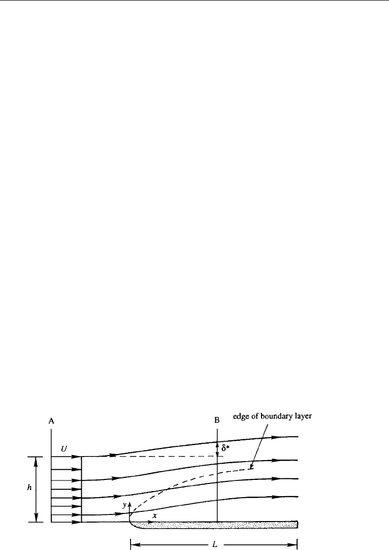
342 Boundary Layers and Related Topics
Figure 10.2 Velocity profiles at two positions within the boundary layer. The velocity arrows are drawn
at the same distance y from the surface, showing that the variation of u with x is of the order of the free
stream velocity U
∞
. The boundary layer thickness is greatly exaggerated.
measure of the first advective term in equation (10.1) is
u
∂u
∂x
∼
U
2
∞
L
, (10.2)
where ∼ is to be interpreted as “of order.” We shall see shortly that the other advec-
tive term in equation (10.1) is of the same order. A measure of the viscous term in
equation (10.1) is
ν
∂
2
u
∂y
2
∼
νU
∞
¯
δ
2
. (10.3)
The magnitude of
¯
δ can now be estimated by noting that the advective and viscous
terms should be of the same order within the boundary layer, if viscous terms are to
be important. Equating equations (10.2) and (10.3), we obtain
¯
δ ∼
νL
U
∞
or
¯
δ
L
∼
1
√
Re
.
This estimate of
¯
δ can also be obtained by using results of unsteady parallel flows
discussed in the preceding chapter, in which we saw that viscous effects diffuse to
a distance of order
√
νt in time t. As the time to flow along a body of length L is
of order L/U
∞
, the width of the diffusive layer at the end of the body is of order
√
νL/U
∞
.
A formal simplification of the equations of motion within the boundary layer
can now be performed. The basic idea is that variations across the boundary layer are
much faster than variations along the layer, that is
∂
∂x
∂
∂y
,
∂
2
∂x
2
∂
2
∂y
2
.
2. Boundary Layer Approximation 343
The distances in the x-direction over which the velocity varies appreciably are of
order L, but those in the y-direction are of order
¯
δ, which is much smaller than L.
Let us first determine a measure of the typical variation of v within the boundary
layer. This can be done from an examination of the continuity equation ∂u/∂x +
∂v/∂y = 0. Because u v and ∂/∂x ∂/∂y, we expect the two terms of the
continuity equation to be of the same order. This requires U
∞
/L ∼ v/
¯
δ, or that the
variations of v are of order
v ∼
¯
δU
∞
/L ∼ U
∞
/
√
Re.
Next we estimate the magnitude of variation of pressure within the boundary
layer. Experimental data on high Reynolds number flows show that the pressure distri-
bution is nearly that in an irrotational flow around the body, implying that the pressure
forces are of the order of the inertia forces. The requirement ∂p/∂x ∼ ρu(∂u/∂x)
shows that the pressure variations within the flow field are of order
p − p
∞
∼ ρU
2
∞
.
The proper nondimensional variables in the boundary layer are therefore
x
=
x
L
,y
=
y
¯
δ
=
y
L
√
Re,
u
=
u
U
∞
,v
=
v
¯
δU
∞
/L
=
v
U
∞
√
Re,p
=
p − p
∞
ρU
2
,
(10.4)
where
¯
δ =
√
νL/U
∞
. The important point to notice is that the distances across
the boundary layer have been magnified or “stretched” by defining y
= y/
¯
δ =
(y/L)
√
Re.
In terms of these nondimensional variables, the complete equations of motion
for the boundary layer are
u
∂u
∂x
+ v
∂u
∂y
=−
∂p
∂x
+
1
Re
∂
2
u
∂x
2
+
∂
2
u
∂y
2
, (10.5)
1
Re
u
∂v
∂x
+ v
∂v
∂y
=−
∂p
∂y
+
1
Re
2
∂
2
v
∂x
2
+
1
Re
∂
2
v
∂y
2
, (10.6)
∂u
∂x
+
∂v
∂y
= 0, (10.7)
where we have defined Re ≡ U
∞
L/ν as an overall Reynolds number. In these
equations, each of the nondimensional variables and their derivatives is of order one.
For example, ∂u
/∂y
∼ 1 in equation (10.5), essentially because the changes in
u
and y
within the boundary layer are each of order one, a consequence of our
normalization (10.4). It follows that the size of each term in the set (10.5) and (10.6)
is determined by the presence of a multiplying factor involving the parameter Re. In
particular, each term in equation (10.5) is of order one except the second term on the
344 Boundary Layers and Related Topics
right-hand side, whose magnitude is of order 1/Re. As Re →∞, these equations
asymptotically become
u
∂u
∂x
+ v
∂u
∂y
=−
∂p
∂x
+
∂
2
u
∂y
2
,
0 =−
∂p
∂y
,
∂u
∂x
+
∂v
∂y
= 0.
The exercise of going through the nondimensionalization has been valuable,
since it has shown what terms drop out under the boundary layer assumption. Trans-
forming back to dimensional variables, the approximate equations of motion within
the boundary layer are
u
∂u
∂x
+ v
∂u
∂y
=−
1
ρ
∂p
∂x
+ ν
∂
2
u
∂y
2
,
0 =−
∂p
∂y
,
∂u
∂x
+
∂v
∂y
=0.
(10.8)
(10.9)
(10.10)
Equation (10.9) says that the pressure is approximately uniform across the bound-
ary layer, an important result. The pressure at the surface is therefore equal to that at
the edge of the boundary layer, and so it can be found from a solution of the irrotational
flow around the body. We say that the pressure is “imposed” on the boundary layer
by the outer flow. This justifies the experimental fact, pointed out in the preceding
section, that the observed surface pressure is approximately equal to that calculated
from the irrotational flow theory. (A vanishing ∂p/∂y, however, is not valid if the
boundary layer separates from the wall or if the radius of curvature of the surface is
not large compared with the boundary layer thickness. This will be discussed later
in the chapter.) The pressure gradient at the edge of the boundary layer can be found
from the inviscid Euler equation
−
1
ρ
dp
dx
= U
e
dU
e
dx
, (10.11)
or from its integral p + ρU
2
e
/2 = constant, which is the Bernoulli equation. This
is because v
e
∼ 1/
√
Re → 0. Here U
e
(x) is the velocity at the edge of the bound-
ary layer (Figure 10.1). This is the matching of the outer inviscid solution with the
boundary layer solution in the overlap domain of common validity. However, instead
of finding dp/dx at the edge of the boundary layer, as a first approximation we
can apply equation (10.11) along the surface of the body, neglecting the existence
of the boundary layer in the solution of the outer problem; the error goes to zero
as the boundary layer becomes increasingly thin. In any event, the dp/dx term in

2. Boundary Layer Approximation 345
equation (10.8) is to be regarded as known from an analysis of the outer problem,
which must be solved before the boundary layer flow can be solved.
Equations (10.8) and (10.10) are then used to determine u and v in the boundary
layer. The boundary conditions are
u(x, 0) = 0, (10.12)
v(x, 0) = 0, (10.13)
u(x, ∞) = U(x), (10.14)
u(x
0
,y) = u
in
(y). (10.15)
Condition (10.14) merely means that the boundary layer must join smoothly with
the inviscid outer flow; points outside the boundary layer are represented by
y =∞, although we mean this strictly in terms of the nondimensional distance
y/
¯
δ = (y/L)
√
Re →∞. Condition (10.15) implies that an initial velocity profile
u
in
(y) at some location x
0
is required for solving the problem. This is because the
presence of the terms u ∂u/∂x and ν∂
2
u/∂y
2
gives the boundary layer equations a
parabolic character, with x playing the role of a timelike variable. Recall the Stokes
problem of a suddenly accelerated plate, discussed in the preceding chapter, where
the equation is ∂u/∂t = ν∂
2
u/∂y
2
. In such problems governed by parabolic equa-
tions, the field at a certain time (or x in the problem here) depends only on its past
history. Boundary layers therefore transfer effects only in the downstream direction.
In contrast, the complete Navier–Stokes equations are of elliptic nature. Elliptic equa-
tions require specification on the bounding surface of the domain of solution. The
Navier–Stokes equations are elliptic in velocity and thus require boundary conditions
on the velocity (or its derivative normal to the boundary) upstream, downstream, and
on the top and bottom boundaries, that is, all around. The upstream influence of the
downstream boundary condition is always of concern in computations.
In summary, the simplifications achieved because of the thinness of the boundary
layer are the following. First, diffusion in the x-direction is negligible compared to that
in the y-direction. Second, the pressure field can be found from the irrotational flow
theory, so that it is regarded as a known quantity in boundary layer analysis. Here, the
boundary layer is so thin that the pressure does not change across it. Further, a crude
estimate of the shear stress at the wall or skin friction is available from knowledge
of the order of the boundary layer thickness τ
0
∼ µU/
¯
δ ∼ (µU /L)
√
Re. The skin
friction coefficient is
τ
0
(1/2)ρU
2
∼
2µU
ρLU
2
√
Re ∼
2
√
Re
.
As we shall see from the solutions to the problems in the following sections, this is
indeed the correct order of magnitude. Only the finite numerical factor differs from
problem to problem.
It is useful to compare equation (10.5) with equation (9.60), where we nondi-
mensionalized both x- and y-directions by the same length scale. Notice that in
equation (9.60) the Reynolds number multiplies both diffusion terms, whereas in
346 Boundary Layers and Related Topics
equation (10.5) the diffusion term in the y-direction has been explicitly made order
one by a normalization appropriate within the boundary layer.
3. Different Measures of Boundary Layer Thickness
As the velocity in the boundary layer smoothly joins that of the outer flow, we have
to decide how to define the boundary layer thickness. The three common measures
are described here.
The u = 0.99U Thickness
One measure of the boundary thickness is the distance from the wall where the
longitudinal velocity reaches 99% of the local free stream velocity, that is where
u = 0.99 U . We shall denote this as δ
99
. This definition of the boundary layer thickness
is however rather arbitrary, as we could very well have chosen the thickness as the
point where u = 0.95 U .
Displacement Thickness
A second measure of the boundary layer thickness, and one in which there is no
arbitrariness, is the displacement thickness δ
∗
. This is defined as the distance by
which the wall would have to be displaced outward in a hypothetical frictionless flow
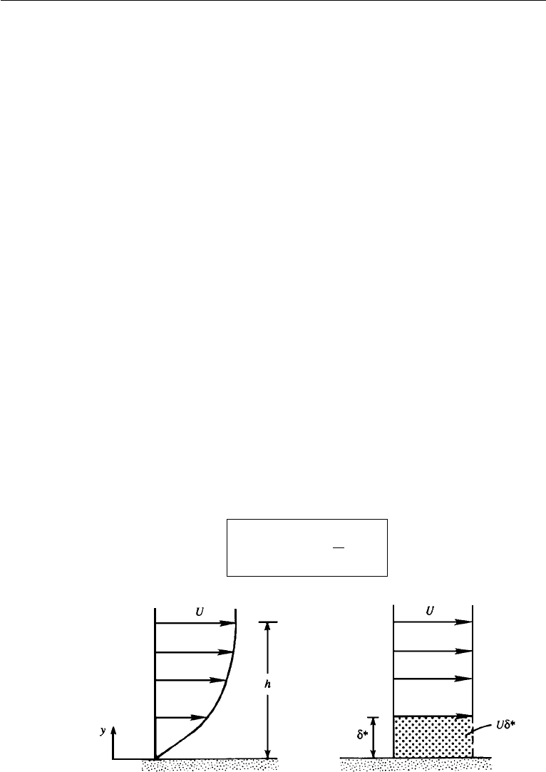
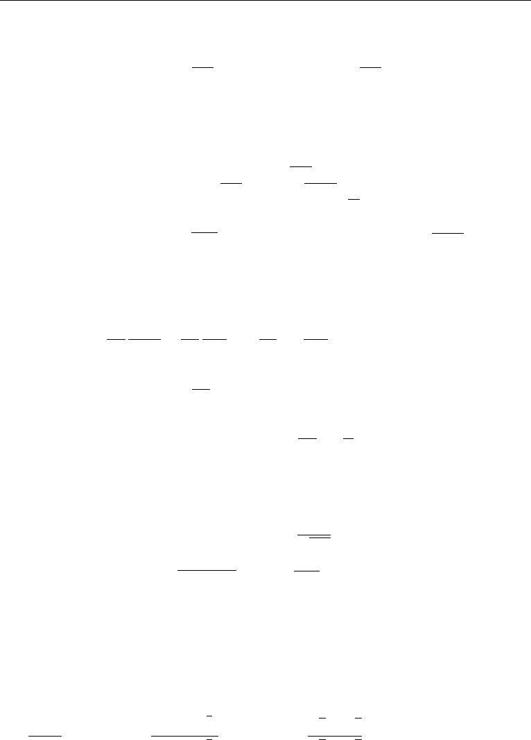
so as to maintain the same mass flux as in the actual flow. Let h be the distance from
the wall to a point far outside the boundary layer (Figure 10.3). From the definition
of δ
∗
, we obtain
h
0
udy = U(h − δ
∗
),
where the left-hand side is the actual mass flux below h and the right-hand side is the
mass flux in the frictionless flow with the walls displaced by δ
∗
. Letting h →∞, the
aforementioned gives
δ
∗
=
∞
0
1 −
u
U
dy.
(10.16)
Figure 10.3 Displacement thickness.
3. Different Measures of Boundary Layer Thickness 347
The upper limit in equation (10.16) may be allowed to extend to infinity because, as
we shall show in the following, u/U → 0 exponentially fast in y as y →∞.
The concept of displacement thickness is used in the design of ducts, intakes of
air-breathing engines, wind tunnels, etc. by first assuming a frictionless flow and then
enlarging the passage walls by the displacement thickness so as to allow the same flow
rate. Another use of δ
∗
is in finding dp/dx at the edge of the boundary layer, needed for
solving the boundary layer equations. The first approximation is to neglect the exis-
tence of the boundary layer, and calculate the irrotational dp/dx over the body surface.
A solution of the boundary layer equations gives the displacement thickness, using
equation (10.16). The body surface is then displaced outward by this amount and a next
approximation of dp/dx is found from a solution of the irrotational flow, and so on.
The displacement thickness can also be interpreted in an alternate and possibly
more illuminating way. We shall now show that it is the distance by which the stream-
lines outside the boundary layer are displaced due to the presence of the boundary
layer. Figure 10.4 shows the displacement of streamlines over a flat plate. Equating
mass flux across two sections A and B, we obtain
Uh =
h+δ
∗
0
udy =
h
0
udy + Uδ
∗
,
which gives
Uδ
∗
=
h
0
(U − u) dy.
Here h is any distance far from the boundary and can be replaced by ∞ without
changing the integral, which then reduces to equation (10.16).
Momentum Thickness
A third measure of the boundary layer thickness is the momentum thickness θ, defined
such that ρU
2
θ is the momentum loss due to the presence of the boundary layer. Again
choose a streamline such that its distance h is outside the boundary layer, and consider
Figure 10.4 Displacement thickness and streamline displacement.

348 Boundary Layers and Related Topics
the momentum flux (=velocity times mass flow rate) below the streamline, per unit
width. At section A the momentum flux is ρU
2
h; that across section B is
h+δ
∗
0
ρu
2
dy =
h
0
ρu
2
dy + ρδ
∗
U
2
.
The loss of momentum due to the presence of the boundary layer is therefore the
difference between the momentum fluxes across A and B, which is defined as ρU
2
θ:
ρU
2
h −
h
0
ρu
2
dy − ρδ
∗
U
2
≡ ρU
2
θ.
Substituting the expression for δ
∗
gives
h
0
(U
2
− u
2
)dy − U
2
h
0
1 −
u
U
dy = U
2
θ,
from which
θ =
∞
0
u
U
1 −
u
U
dy,
(10.17)
where we have replaced h by ∞ because u = U for y>h.
4. Boundary Layer on a Flat Plate with a Sink at
the Leading Edge: Closed Form Solution
Although all other texts start their boundary layer discussion with the uniform flow
over a semi-infinite flat plate, there is an even simpler related problem that can be
solved in closed form in terms of elementary functions. We shall consider the large
Reynolds number flow generated by a sink at the leading edge of a flat plate. The outer
inviscid flow is represented by ψ = mθ/2π , m<0 so that u
r
= m/2πr, u
θ
= 0
[Chapter 6, Section 5, equation (6.24) and Figure 6.6]. This represents radially inward
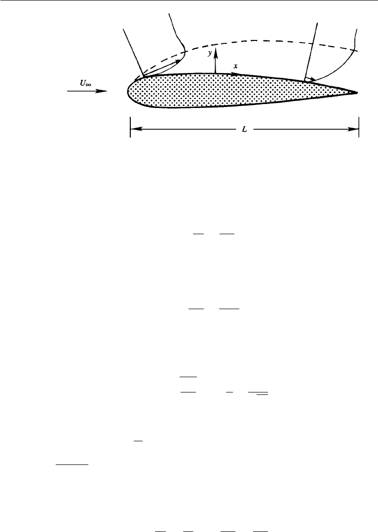
flow towards the origin. A flat plate is now aligned with the x-axis so that its boundary
is represented by θ = 0. For large Re, the boundary layer is thin so x = r cos θ ≈ r
because θ 1. For simplicity in what follows we shall absorb the 2π into the m
by defining m
= m/2π and then suppressing the prime. The velocity at the edge
of the boundary layer is U
e
(x) = m/x, m<0 and the local Reynolds number is
U
e
(x)x/ν = m/ν = Re
x
. Boundary layer coordinates are used, as in Figure 10.1,
with y normal to the plate and the origin at the leading edge.
The boundary layer equations (10.8)–(10.10) with equation (10.11) become
∂u
∂x
+
∂v
∂y
= 0,u
∂u
∂x
+ v
∂u
∂y
=−
m
2
x
3
+ ν
∂
2
u
∂y
2
with the boundary conditions (10.12)–(10.15). We consider the limiting case Re
x
=
|m/ν|→∞. Because m<0, the flow is from right (larger x) to left (smaller x),
4. Boundary Layer on a Flat Plate with a Sink at the Leading Edge: Closed Form Solution 349
and the initial condition at x = x
0
is specified upstream, that is, at the largest x. The
solution is then determined for all x<x
0
, that is, downstream of the initial location.
The natural way to make the variables dimensionless and finite in the boundary layer
is to normalize x by x
0
, y by x
0
/
√
Re
x
, u by m/x
0
, v by m/(x
0
√
Re
x
). The problem
is fully two-dimensional and well posed for any reasonable initial condition (10.15).
Now, suppress the initial condition. The length scale x
0
, crucial to rendering the
problem properly dimensionless, has disappeared. How is one to construct a dimen-
sionless formulation? We have seen before that this situation results in a reduction in
the dimensionality of the space required for the solution. The variable y can be made
dimensionless only by x and must be stretched by
√
Re
x
to be finite in the boundary
layer. The unique choice is then (y/x)
√
Re
x
= (y/x)
√
|m/ν|=η. This is consistent
with the similarity variable for Stokes’ first problem η = y/
√
νt when t is taken to
be x/U and U = m/x. Finite numerical factors are irrelevant here. Further, we note
that we have found that δ ∼ x
0
/
Re
x
0
so with the x
0
scale absent, δ ∼ x
√
|m/ν|
and η = y/δ. Next we will reduce mass and momentum conservation to an ordinary
differential equation for the xsimilarity streamfunction. To reverse the flow we will
define the streamfunction ψ via u =−∂ψ/∂y, v = ∂ψ/∂x (note sign change). We
now have:
∂ψ
∂y
∂
2
ψ
∂y ∂x
−
∂ψ
∂x
∂
2
ψ
∂y
2
=−
m
2
x
3
− ν
∂
3
ψ
∂y
3
,
y = 0: ψ =
∂ψ
∂y
= 0,
y → overlap with inviscid flow:
∂ψ
∂y
→
m
x
.
The streamfunction is made dimensionless by its order of magnitude and put in
similarity form via
ψ(x, y) = U
e
δ(x)f (η) = U
e
(x) ·
x
√
Re
x
f(η)
=
νU
e
(x) · xf (η) =
|νm|f(η),
in this problem. The problem for f reduces to
f
(η) − f
2
=−1,
f(0) = 0,f
(0) = 0,f
(∞) = 1.
This may be solved in closed form with the result
u
U
e
(x)
= f
(η) = 3
1 − αe
−
√
2η
1 + αe
−
√
2η
2
− 2,α=
√
3 −
√
2
√
3 +
√
2
= 0.101 ....

350 Boundary Layers and Related Topics
A result equivalent to this was first obtained by Pohlhausen (1921) in his solution
for flow in a convergent channel. From this simple solution we can establish several
properties characteristic of laminar boundary layers. First, as η →∞, the matching
with the inviscid solution occurs exponentially fast, as f
(η) ∼ 1 − 12αe
−
√
2η
+
smaller terms as η →∞.
Next v/U
e
is of the correct small order,
v
U
e
=
y
x
f
(η) =
1
√
Re
x
ηf
(η) ∼
1
√
Re
x
.
The behavior of the displacement thickness is obtained from the definition
δ
∗
=
∞
0
1 −
u
U
e
dy =
∞
0
[1 − f
(η)]dη ·
x
√
Re
x
,
δ
∗
x
=
1
√
Re
x
∞
0
[1 − f
(η)]dη =
12α
[(1 + α)
√
2
√
Re
x
]
=
0.7785
√
Re
x
∼
1
√
Re
x
.
The shear stress at the wall is
τ
0
= µ
∂u
∂y
0
=−µ
m
x
2
m
ν
f
(0), f
(0) =
2
√
3
.
Then the skin friction coefficient is
C
f
=
τ
0
(1/2)ρU
2
e
=
−4/
√
3
√
Re
x
, Re
x
=
m
ν
.
Aside from numerical factors, which are obviously problem specific, the preced-
ing results are universally valid for all similarity solutions of the laminar bound-
ary layer equations. U
e
(x) is the velocity at the edge of the boundary layer and
Re
x
= U
e
(x)x/ν. In these terms
η =
y
x
Re
x
, ψ (x, y) =
νU
e
(x) · x f (η),
f(η) = u/U
e
(x) → 1 exponentially fast as η →∞. We find v/U
e
∼ 1/
√
Re
x
,
δ
∗
/x ∼ 1/
√
Re
x
,C
f
∼ 1/
√
Re
x
.
Axisymmetric Problem
Now let us consider the axially symmetric version of the problem we just solved.
This is the flow in the neighborhood of an infinite flat plate generated by a sink
in the center of the plate. The inviscid outer flow is u
r
=−Q/r
2
where r is the
spherical radial coordinate centered on the sink. The boundary layer adjacent to the
plate is best treated in cylindrical coordinates r, θ , z with ∂/∂θ = 0 (see Figure 10.5).
Mass conservation for a constant density flow with symmetry about the z-axis is
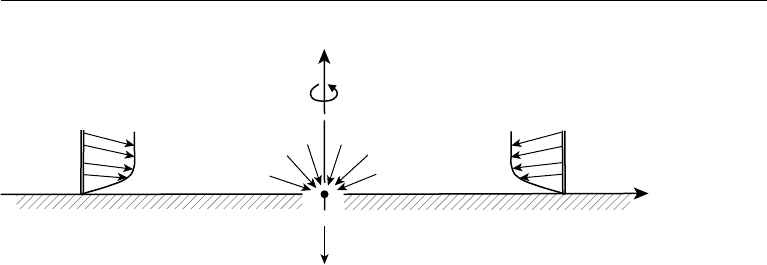
4. Boundary Layer on a Flat Plate with a Sink at the Leading Edge: Closed Form Solution 351
z
θ
r,x
Figure 10.5 Axisymmetric flow into a sink at the center of an infinite plate.
∂/∂r(ru
r
) + ∂/∂z(ru
z
) = 0. In the following, the streamwise coordinate r is replaced
by x. Since U
e
=−Q/x
2
, the local Reynolds number can be written as Re
x
=
U
e
x/ν = Q/xν. Assuming this is sufficiently large, the full Navier–Stokes equations
reduce to the boundary layer equations with an error that is small in powers of inverse
Re
x
. Thus we seek to solve
u∂u/∂x + w∂u/∂z = U
e
dU
e
/dx + ν∂
2
u/∂z
2
subject to u = w = 0onz = 0 and u → U
e
as z leaves the boundary layer.
A similarity solution can be obtained provided the requirement for an initial velocity
distribution is not imposed. First, the streamwise momentum equation is put in terms
of the axisymmetric streamfunction, u =−(1
θ
/x) ×∇ψ, so that xu =−∂ψ/∂z,
xw = ∂ψ/∂x. With the modification of the streamfunction due to axial symmetry,
the universal dimensionless similarity form becomes
ψ(x,z) = x[νxU
e
(x)]
1/2
f(η)= (νQx)
1/2
f(η)
where η = (z/x)(Re
x
)
1/2
= (Q/ν)
1/2
z/x
3/2
. The velocity components trans-
form to u =−x
−1
∂ψ/∂z = U
e
f
(η), w =[(νQ)
1/2
/(2x
3/2
)](f − 3ηf
) =
{U
e
/[2(Re
x
)
1/2
]}(f − 3ηf
).
The streamwise momentum equation transforms to
f
− (1/2)ff
+ 2(1 − f
2
) = 0
subject to (10.18)
f(0) = 0,f
(0) = 0,f
(∞) = 1.
Rosenhead provides a tabulation of the solution to f
− ff
+ 4(1 − f
2
) = 0,
which is related to the equation above by the scaling η/2
1/2
, and f/2
1/2
.(Wehave
tried not to add extraneous numerical factors to our universal dimensionless similarity
scaling.) The solution to (10.18) is displayed in Figure 10.6.