Brealey, Myers. Principles of Corporate Finance. 7th edition

Подождите немного. Документ загружается.

Brealey−Meyers:

Principles of Corporate

Finance, Seventh Edition

II. Risk 9. Capital Budgeting and

Risk

Companies, 2003

Step 1, then, is to do your best to make unbiased forecasts of a project’s cash

flows. Step 2 is to consider whether investors would regard the project as more or

less risky than typical for a company or division. Here our advice is to search for

characteristics of the asset that are associated with high or low betas. We wish we

had a more fundamental scientific understanding of what these characteristics are.

We see business risks surfacing in capital markets, but as yet there is no satisfac-

tory theory describing how these risks are generated. Nevertheless, some things

are known.

What Determines Asset Betas?

Cyclicality Many people intuitively associate risk with the variability of book, or

accounting, earnings. But much of this variability reflects unique or diversifiable

risk. Lone prospectors in search of gold look forward to extremely uncertain future

earnings, but whether they strike it rich is not likely to depend on the performance

of the market portfolio. Even if they do find gold, they do not bear much market

risk. Therefore, an investment in gold has a high standard deviation but a relatively

low beta.

What really counts is the strength of the relationship between the firm’s earn-

ings and the aggregate earnings on all real assets. We can measure this either by the

accounting beta or by the cash-flow beta. These are just like a real beta except that

changes in book earnings or cash flow are used in place of rates of return on secu-

rities. We would predict that firms with high accounting or cash-flow betas should

also have high stock betas—and the prediction is correct.

This means that cyclical firms—firms whose revenues and earnings are strongly

dependent on the state of the business cycle—tend to be high-beta firms. Thus you

should demand a higher rate of return from investments whose performance is

strongly tied to the performance of the economy.

Operating Leverage We have already seen that financial leverage (i.e., the com-

mitment to fixed-debt charges) increases the beta of an investor’s portfolio. In just

the same way, operating leverage (i.e., the commitment to fixed production charges)

must add to the beta of a capital project. Let’s see how this works.

The cash flows generated by any productive asset can be broken down into rev-

enue, fixed costs, and variable costs:

Cash flow ⫽ revenue ⫺ fixed cost ⫺ variable cost

Costs are variable if they depend on the rate of output. Examples are raw materi-

als, sales commissions, and some labor and maintenance costs. Fixed costs are cash

outflows that occur regardless of whether the asset is active or idle (e.g., property

taxes or the wages of workers under contract).

We can break down the asset’s present value in the same way:

PV(asset) ⫽ PV(revenue) ⫺ PV(fixed cost) ⫺ PV(variable cost)

Or equivalently

PV(revenue) ⫽ PV(fixed cost) ⫹ PV(variable cost) ⫹ PV(asset)

CHAPTER 9

Capital Budgeting and Risk 237

For example, see W. H. Beaver and J. Manegold, “The Association between Market-Determined and

Accounting-Determined Measures of Systematic Risk: Some Further Evidence,” Journal of Financial and

Quantitative Analysis 10 (June 1979), pp. 231–284.

Brealey−Meyers:

Principles of Corporate

Finance, Seventh Edition

II. Risk 9. Capital Budgeting and

Risk

Companies, 2003

Those who receive the fixed costs are like debtholders in the project; they simply get

a fixed payment. Those who receive the net cash flows from the asset are like hold-

ers of common stock; they get whatever is left after payment of the fixed costs.

We can now figure out how the asset’s beta is related to the betas of the values

of revenue and costs. We just use our previous formula with the betas relabeled:

In other words, the beta of the value of the revenues is simply a weighted average

of the beta of its component parts. Now the fixed-cost beta is zero by definition:

Whoever receives the fixed costs holds a safe asset. The betas of the revenues and

variable costs should be approximately the same, because they respond to the same

underlying variable, the rate of output. Therefore, we can substitute ␤

variable cost

and solve for the asset beta. Remember that ␤

fixed cost

⫽ 0.

Thus, given the cyclicality of revenues (reflected in ␤

revenue

), the asset beta is propor-

tional to the ratio of the present value of fixed costs to the present value of the project.

Now you have a rule of thumb for judging the relative risks of alternative de-

signs or technologies for producing the same project. Other things being equal, the

alternative with the higher ratio of fixed costs to project value will have the higher

project beta. Empirical tests confirm that companies with high operating leverage

actually do have high betas.

Searching for Clues

Recent research suggests a variety of other factors that affect an asset’s beta.

But

going through a long list of these possible determinants would take us too far

afield.

You cannot hope to estimate the relative risk of assets with any precision, but good

managers examine any project from a variety of angles and look for clues as to its risk-

iness. They know that high market risk is a characteristic of cyclical ventures and of

projects with high fixed costs. They think about the major uncertainties affecting the

economy and consider how projects are affected by these uncertainties.

⫽␤

revenue

c1 ⫹

PV1fixed cost2

PV1asset2

␤

assets

⫽␤

revenue

PV1revenue2⫺ PV1variable cost2

PV1asset2

⫹␤

variable cost

PV1variable cost2

PV1revenue2

⫹␤

asset

PV1asset2

PV1revenue2

␤

revenue

⫽␤

fixed cost

PV1fixed cost2

PV1revenue2

238 PART II Risk

See B. Lev, “On the Association between Operating Leverage and Risk,” Journal of Financial and Quan-

titative Analysis 9 (September 1974), pp. 627–642; and G. N. Mandelker and S. G. Rhee, “The Impact of

the Degrees of Operating and Financial Leverage on Systematic Risk of Common Stock,” Journal of Fi-

nancial and Quantitative Analysis 19 (March 1984), pp. 45–57.

This work is reviewed in G. Foster, Financial Statement Analysis, 2d ed., Prentice-Hall, Inc., Englewood

Cliffs, N.J., 1986, chap. 10.

Sharpe’s article on a “multibeta” interpretation of market risk offers a useful way of thinking about

these uncertainties and tracing their impact on a firm’s or project’s risk. See W. F. Sharpe, “The Capital

Asset Pricing Model: A ‘Multi-Beta’ Interpretation,” in H. Levy and M. Sarnat (eds.), Financial Decision

Making under Uncertainty, Academic Press, New York, 1977.

Brealey−Meyers:

Principles of Corporate

Finance, Seventh Edition

II. Risk 9. Capital Budgeting and

Risk

Companies, 2003

In practical capital budgeting, a single discount rate is usually applied to all future

cash flows. For example, the financial manager might use the capital asset pricing

model to estimate the cost of capital and then use this figure to discount each year’s

expected cash flow.

Among other things, the use of a constant discount rate assumes that project risk

does not change.

We know that this can’t be strictly true, for the risks to which

companies are exposed are constantly shifting. We are venturing here onto some-

what difficult ground, but there is a way to think about risk that can suggest a route

through. It involves converting the expected cash flows to certainty equivalents.

We will first explain what certainty equivalents are. Then we will use this knowl-

edge to examine when it is reasonable to assume constant risk. Finally we will

value a project whose risk does change.

Think back to the simple real estate investment that we used in Chapter 2 to intro-

duce the concept of present value. You are considering construction of an office build-

ing that you plan to sell after one year for $400,000. Since that cash flow is uncertain,

you discount at a risk-adjusted discount rate of 12 percent rather than the 7 percent

risk-free rate of interest. This gives a present value of 400,000/1.12 ⫽ $357,143.

Suppose a real estate company now approaches and offers to fix the price at

which it will buy the building from you at the end of the year. This guarantee

would remove any uncertainty about the payoff on your investment. So you would

accept a lower figure than the uncertain payoff of $400,000. But how much less? If

the building has a present value of $357,143 and the interest rate is 7 percent, then

In other words, a certain cash flow of $382,143 has exactly the same present

value as an expected but uncertain cash flow of $400,000. The cash flow of $382,143

is therefore known as the certainty-equivalent cash flow. To compensate for both the

delayed payoff and the uncertainty in real estate prices, you need a return of

400,000 ⫺ 357,143 ⫽ $42,857. To get rid of the risk, you would be prepared to take

a cut in the return of 400,000 ⫺ 382,143 ⫽ $17,857.

Our example illustrates two ways to value a risky cash flow C

Method 1: Discount the risky cash flow at a risk-adjusted discount rate r that is

greater than r

The risk-adjusted discount rate adjusts for both time and risk.

This is illustrated by the clockwise route in Figure 9.5.

Method 2: Find the certainty-equivalent cash flow and discount at the risk-free

interest rate r

. When you use this method, you need to ask, What is the

smallest certain payoff for which I would exchange the risky cash flow C

Certain cash flow ⫽ $382,143

PV ⫽

Certain cash flow

1.07

⫽ $357,143

CHAPTER 9 Capital Budgeting and Risk 239

9.6 ANOTHER LOOK AT RISK AND DISCOUNTED

CASH FLOW

See E. F. Fama, “Risk-Adjusted Discount Rates and Capital Budgeting under Uncertainty,” Journal of

Financial Economics 5 (August 1977), pp. 3–24; or S. C. Myers and S. M. Turnbull, “Capital Budgeting

and the Capital Asset Pricing Model: Good News and Bad News,” Journal of Finance 32 (May 1977),

pp. 321–332.

The quantity r can be less than r

for assets with negative betas. But the betas of the assets that corpo-

rations hold are almost always positive.

Brealey−Meyers:

Principles of Corporate

Finance, Seventh Edition

II. Risk 9. Capital Budgeting and

Risk

Companies, 2003

This is called the certainty equivalent of C

denoted by CEQ

Since CEQ

the value equivalent of a safe cash flow, it is discounted at the risk-free rate.

The certainty-equivalent method makes separate adjustments for risk and time.

This is illustrated by the counterclockwise route in Figure 9.5.

We now have two identical expressions for PV:

For cash flows two, three, or t years away,

When to Use a Single Risk-Adjusted Discount Rate for Long-Lived Assets

We are now in a position to examine what is implied when a constant risk-adjusted

discount rate, r, is used to calculate a present value.

Consider two simple projects. Project A is expected to produce a cash flow of

$100 million for each of three years. The risk-free interest rate is 6 percent, the mar-

ket risk premium is 8 percent, and project A’s beta is .75. You therefore calculate A’s

opportunity cost of capital as follows:

Discounting at 12 percent gives the following present value for each cash flow:

⫽ 6 ⫹ .75182⫽ 12%

r ⫽ r

⫹␤1r

⫺ r

PV ⫽

11 ⫹ r2

⫽

CEQ

11 ⫹ r

PV ⫽

1 ⫹ r

⫽

CEQ

1 ⫹ r

240 PART II Risk

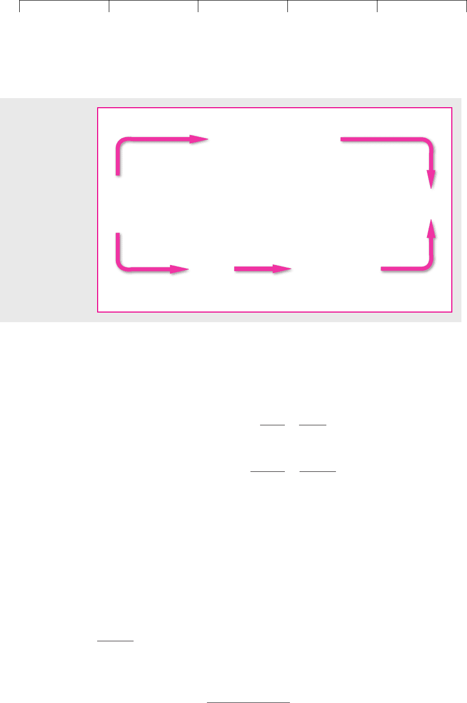
Risk-Adjusted Discount Rate Method

Certainty-Equivalent Method

Discount for time and risk

Present

value

Future

cash

flow

Discount for time

value of money

Haircut

for risk

FIGURE 9.5

Two ways to

calculate present

value. “Haircut for

risk” refers to the

reduction of the cash

flow from its fore-

casted value to its

certainty equivalent.

CEQ

can be calculated directly from the capital asset pricing model. The certainty-equivalent form

of the CAPM states that the certainty-equivalent value of the cash flow, C

, is PV ⫽ C

⫺␭cov(

, ˜r

Cov (

, ˜r

) is the covariance between the uncertain cash flow,

, and the return on the market, r

Lambda, ␭, is a measure of the market price of risk. It is defined as (r

⫺ r

)/␴

. For example, if r

⫺

⫽ .08 and the standard deviation of market returns is ␴

⫽ .20, then lambda ⫽ .08/.20

⫽ 2. We show

on the Brealey-Myers website (www.mhhe.com/bm7e) how the CAPM formula can be twisted around

into this certainty-equivalent form.

Brealey−Meyers:

Principles of Corporate

Finance, Seventh Edition

II. Risk 9. Capital Budgeting and

Risk

Companies, 2003

CHAPTER 9 Capital Budgeting and Risk 241

Project A

Year Cash Flow PV at 12%

1 100 89.3

2 100 79.7

3 100 71.2

Total PV 240.2

Now compare these figures with the cash flows of project B. Notice that B’s cash

flows are lower than A’s; but B’s flows are safe, and therefore they are discounted

at the risk-free interest rate. The present value of each year’s cash flow is identical

for the two projects.

Project B

Year Cash Flow PV at 6%

1 94.6 89.3

2 89.6 79.7

3 84.8 71.2

Total PV 240.2

In year 1 project A has a risky cash flow of 100. This has the same PV as the safe

cash flow of 94.6 from project B. Therefore 94.6 is the certainty equivalent of 100.

Since the two cash flows have the same PV, investors must be willing to give up

100 ⫺ 94.6 ⫽ 5.4 in expected year-1 income in order to get rid of the uncertainty.

In year 2 project A has a risky cash flow of 100, and B has a safe cash flow of 89.6.

Again both flows have the same PV. Thus, to eliminate the uncertainty in year 2,

investors are prepared to give up 100 ⫺ 89.6 ⫽ 10.4 of future income. To eliminate

uncertainty in year 3, they are willing to give up 100 ⫺ 84.8 ⫽ 15.2 of future income.

To value project A, you discounted each cash flow at the same risk-adjusted dis-

count rate of 12 percent. Now you can see what is implied when you did that. By

using a constant rate, you effectively made a larger deduction for risk from the later

cash flows:

Forecasted Certainty-

Cash Flow for Equivalent Deduction

Year Project A Cash Flow for Risk

1 100 94.6 5.4

2 100 89.6 10.4

3 100 84.8 15.2

The second cash flow is riskier than the first because it is exposed to two years of mar-

ket risk. The third cash flow is riskier still because it is exposed to three years of mar-

ket risk. This increased risk is reflected in the steadily declining certainty equivalents:

Forecasted Certainty-

Cash Flow for Equivalent Ratio of CEQ

Year Project A (C

) Cash Flow (CEQ

) to C

1 100 94.6 .946

2 100 89.6 .896 ⫽ .946

3 100 84.8 .848 ⫽ .946

Brealey−Meyers:

Principles of Corporate

Finance, Seventh Edition

II. Risk 9. Capital Budgeting and

Risk

Companies, 2003

Our example illustrates that if we are to use the same discount rate for every future

cash flow, then the certainty equivalents must decline steadily as a fraction of the cash

flow. There’s no law of nature stating that certainty equivalents have to decrease in

this smooth and regular way. It may be a fair assumption for most projects most of the

time, but we’ll sketch in a moment a real example in which that is not the case.

A Common Mistake

You sometimes hear people say that because distant cash flows are riskier, they

should be discounted at a higher rate than earlier cash flows. That is quite wrong: We

have just seen that using the same risk-adjusted discount rate for each year’s cash

flow implies a larger deduction for risk from the later cash flows. The reason is that

the discount rate compensates for the risk borne per period. The more distant the cash

flows, the greater the number of periods and the larger the total risk adjustment.

When You Cannot Use a Single Risk-Adjusted Discount Rate

for Long-Lived Assets

Sometimes you will encounter problems where risk does change as time passes, and

the use of a single risk-adjusted discount rate will then get you into trouble. For ex-

ample, later in the book we will look at how options are valued. Because an option’s

risk is continually changing, the certainty-equivalent method needs to be used.

Here is a disguised, simplified, and somewhat exaggerated version of an actual

project proposal that one of the authors was asked to analyze. The scientists at Veg-

etron have come up with an electric mop, and the firm is ready to go ahead with pi-

lot production and test marketing. The preliminary phase will take one year and cost

$125,000. Management feels that there is only a 50 percent chance that pilot produc-

tion and market tests will be successful. If they are, then Vegetron will build a $1 mil-

lion plant that would generate an expected annual cash flow in perpetuity of $250,000

a year after taxes. If they are not successful, the project will have to be dropped.

The expected cash flows (in thousands of dollars) are

Management has little experience with consumer products and considers this a

project of extremely high risk.

Therefore management discounts the cash flows

at 25 percent, rather than at Vegetron’s normal 10 percent standard:

This seems to show that the project is not worthwhile.

Management’s analysis is open to criticism if the first year’s experiment resolves a

high proportion of the risk. If the test phase is a failure, then there’s no risk at all—the

project is certain to be worthless. If it is a success, there could well be only normal risk

from then on. That means there is a 50 percent chance that in one year Vegetron will

NPV ⫽⫺125 ⫺

500

1.25

⫹

∞

t⫽2

125

11.252

⫽⫺125, or ⫺$125,000

⫽ .512502⫹ .5102⫽ 125

for t ⫽ 2, 3,

…

⫽ 50% chance of 250 and 50% chance of 0

⫽ .51⫺1,0002⫹ .5102⫽⫺500

⫽ 50% chance of ⫺1,000 and 50% chance of 0

⫽⫺125

242 PART II Risk

We will assume that they mean high market risk and that the difference between 25 and 10 percent is

not a fudge factor introduced to offset optimistic cash-flow forecasts.

Brealey−Meyers:

Principles of Corporate

Finance, Seventh Edition

II. Risk 9. Capital Budgeting and

Risk

Companies, 2003

CHAPTER 9 Capital Budgeting and Risk 243

have the opportunity to invest in a project of normal risk, for which the normal dis-

count rate of 10 percent would be appropriate. Thus the firm has a 50 percent chance

to invest $1 million in a project with a net present value of $1.5 million:

Success

—→ (50% chance)

Pilot production

and market tests

Failure —→ NPV ⫽ 0 (50% chance)

Thus we could view the project as offering an expected payoff of .5(1,500)⫹.5(0) ⫽

750, or $750,000, at t ⫽ 1 on a $125,000 investment at t ⫽ 0. Of course, the certainty

equivalent of the payoff is less than $750,000, but the difference would have to be very

large to justify rejecting the project. For example, if the certainty equivalent is half the

forecasted cash flow and the risk-free rate is 7 percent, the project is worth $225,500:

This is not bad for a $125,000 investment—and quite a change from the negative-

NPV that management got by discounting all future cash flows at 25 percent.

⫽⫺125 ⫹

.517502

1.07

⫽ 225.5, or $225,500

NPV ⫽ C

⫹

CEQ

1 ⫹ r

NPV ⫽⫺1000 ⫹

250

.10

⫽⫹1,500

SUMMARY

In Chapter 8 we set out some basic principles for valuing risky assets. In this chap-

ter we have shown you how to apply these principles to practical situations.

The problem is easiest when you believe that the project has the same market

risk as the company’s existing assets. In this case, the required return equals the re-

quired return on a portfolio of all the company’s existing securities. This is called

the company cost of capital.

Common sense tells us that the required return on any asset depends on its risk.

In this chapter we have defined risk as beta and used the capital asset pricing

model to calculate expected returns.

The most common way to estimate the beta of a stock is to figure out how the

stock price has responded to market changes in the past. Of course, this will give

you only an estimate of the stock’s true beta. You may get a more reliable figure if

you calculate an industry beta for a group of similar companies.

Suppose that you now have an estimate of the stock’s beta. Can you plug that

into the capital asset pricing model to find the company’s cost of capital? No, the

stock beta may reflect both business and financial risk. Whenever a company bor-

rows money, it increases the beta (and the expected return) of its stock. Remember,

the company cost of capital is the expected return on a portfolio of all the firm’s se-

curities, not just the common stock. You can calculate it by estimating the expected

return on each of the securities and then taking a weighted average of these sepa-

rate returns. Or you can calculate the beta of the portfolio of securities and then

plug this asset beta into the capital asset pricing model.

The company cost of capital is the correct discount rate for projects that have the

same risk as the company’s existing business. Many firms, however, use the com-

pany cost of capital to discount the forecasted cash flows on all new projects. This

Visit us at www.mhhe.com/bm7e

Brealey−Meyers:

Principles of Corporate

Finance, Seventh Edition

II. Risk 9. Capital Budgeting and

Risk

Companies, 2003

There is a good review article by Rubinstein on the application of the capital asset pricing model to

capital investment decisions:

M. E. Rubinstein: “A Mean-Variance Synthesis of Corporate Financial Theory,” Journal of Fi-

nance, 28:167–182 (March 1973).

There have been a number of studies of the relationship between accounting data and beta. Many of

these are reviewed in:

G. Foster: Financial Statement Analysis, 2nd ed., Prentice-Hall, Inc., Englewood Cliffs,

N.J., 1986.

244 PART II Risk

is a dangerous procedure. In principle, each project should be evaluated at its own

opportunity cost of capital; the true cost of capital depends on the use to which the

capital is put. If we wish to estimate the cost of capital for a particular project, it is

project risk that counts. Of course the company cost of capital is fine as a discount

rate for average-risk projects. It is also a useful starting point for estimating dis-

count rates for safer or riskier projects.

These basic principles apply internationally, but of course there are complications.

The risk of a stock or real asset may depend on who’s investing. For example, a Swiss

investor would calculate a lower beta for Merck than an investor in the United States.

Conversely, the U.S. investor would calculate a lower beta for a Swiss pharmaceuti-

cal company than a Swiss investor. Both investors see lower risk abroad because of

the less-than-perfect correlation between the two countries’ markets.

If all investors held the world market portfolio, none of this would matter. But there

is a strong home-country bias. Perhaps some investors stay at home because they re-

gard foreign investment as risky. We suspect they confuse total risk with market risk.

For example, we showed examples of countries with extremely volatile stock mar-

kets. Most of these markets were nevertheless low-beta investments for an investor

holding the U.S. market. Again, the reason was low correlation between markets.

Then we turned to the problem of assessing project risk. We provided several

clues for managers seeking project betas. First, avoid adding fudge factors to dis-

count rates to offset worries about bad project outcomes. Adjust cash-flow forecasts

to give due weight to bad outcomes as well as good; then ask whether the chance of

bad outcomes adds to the project’s market risk. Second, you can often identify the

characteristics of a high- or low-beta project even when the project beta cannot be cal-

culated directly. For example, you can try to figure out how much the cash flows are

affected by the overall performance of the economy: Cyclical investments are gener-

ally high-beta investments. You can also look at the project’s operating leverage:

Fixed production charges work like fixed debt charges; that is, they increase beta.

There is one more fence to jump. Most projects produce cash flows for several

years. Firms generally use the same risk-adjusted rate to discount each of these

cash flows. When they do this, they are implicitly assuming that cumulative risk

increases at a constant rate as you look further into the future. That assumption is

usually reasonable. It is precisely true when the project’s future beta will be con-

stant, that is, when risk per period is constant.

But exceptions sometimes prove the rule. Be on the alert for projects where risk

clearly does not increase steadily. In these cases, you should break the project into

segments within which the same discount rate can be reasonably used. Or you

should use the certainty-equivalent version of the DCF model, which allows sepa-

rate risk adjustments to each period’s cash flow.

FURTHER

READING

Visit us at www.mhhe.com/bm7e

Brealey−Meyers:

Principles of Corporate

Finance, Seventh Edition

II. Risk 9. Capital Budgeting and

Risk

Companies, 2003

CHAPTER 9 Capital Budgeting and Risk 245

For some ideas on how one might break down the problem of estimating beta, see:

W. F. Sharpe: “The Capital Asset Pricing Model: A ‘Multi-Beta’ Interpretation,” in H. Levy and

M. Sarnat (eds.), Financial Decision Making under Uncertainty, Academic Press, New York, 1977.

Fama and French present estimates of industry costs of equity capital from both the CAPM and APT

models. The difficulties in obtaining precise estimates are discussed in:

E. F. Fama and K. R. French, “Industry Costs of Equity,” Journal of Financial Economics,

43:153–193 (February 1997).

The assumptions required for use of risk-adjusted discount rates are discussed in:

E. F. Fama: “Risk-Adjusted Discount Rates and Capital Budgeting under Uncertainty,” Jour-

nal of Financial Economics, 5:3–24 (August 1977).

S. C. Myers and S. M. Turnbull: “Capital Budgeting and the Capital Asset Pricing Model:

Good News and Bad News,” Journal of Finance, 32:321–332 (May 1977).

QUIZ

Visit us at www.mhhe.com/bm7e

1. Suppose a firm uses its company cost of capital to evaluate all projects. Will it underes-

timate or overestimate the value of high-risk projects?

2. “A stock’s beta can be estimated by plotting past prices against the level of the market in-

dex and drawing the line of best fit. Beta is the slope of this line.” True or false? Explain.

3. Look back to the top-right panel of Figure 9.2. What proportion of Dell’s return was ex-

plained by market movements? What proportion was unique or diversifiable risk?

How does the unique risk show up in the plot? What is the range of possible error in

the beta estimate?

4. A company is financed 40 percent by risk-free debt. The interest rate is 10 percent, the

expected market return is 18 percent, and the stock’s beta is .5. What is the company

cost of capital?

5. The total market value of the common stock of the Okefenokee Real Estate Company is

$6 million, and the total value of its debt is $4 million. The treasurer estimates that the

beta of the stock is currently 1.5 and that the expected risk premium on the market is

9 percent. The Treasury bill rate is 8 percent. Assume for simplicity that Okefenokee

debt is risk-free.

a. What is the required return on Okefenokee stock?

b. What is the beta of the company’s existing portfolio of assets?

c. Estimate the company cost of capital.

d. Estimate the discount rate for an expansion of the company’s present business.

e. Suppose the company wants to diversify into the manufacture of rose-colored

spectacles. The beta of unleveraged optical manufacturers is 1.2. Estimate the

required return on Okefenokee’s new venture.

6. Nero Violins has the following capital structure:

Total Market Value,

Security Beta $ millions

Debt 0 100

Preferred stock .20 40

Common stock 1.20 200

a. What is the firm’s asset beta (i.e., the beta of a portfolio of all the firm’s securities)?

b. How would the asset beta change if Nero issued an additional $140 million of

common stock and used the cash to repurchase all the debt and preferred stock?

c. Assume that the CAPM is correct. What discount rate should Nero set for

investments that expand the scale of its operations without changing its asset beta?

Assume a risk-free interest rate of 5 percent and a market risk premium of 6 percent.

Brealey−Meyers:

Principles of Corporate

Finance, Seventh Edition

II. Risk 9. Capital Budgeting and

Risk

Companies, 2003

246 PART II Risk

7. True or false?

a. Many foreign stock markets are much more volatile than the U.S. market.

b. The betas of most foreign stock markets (calculated relative to the U.S. market) are

usually greater than 1.0.

c. Investors concentrate their holdings in their home countries. This means that

companies domiciled in different countries may calculate different discount rates

for the same project.

8. Which of these companies is likely to have the higher cost of capital?

a. A’s sales force is paid a fixed annual rate; B’s is paid on a commission basis.

b. C produces machine tools; D produces breakfast cereal.

9. Select the appropriate phrase from within each pair of brackets: “In calculating PV there

are two ways to adjust for risk. One is to make a deduction from the expected cash flows.

This is known as the [certainty-equivalent; risk-adjusted discount rate] method. It is usu-

ally written as PV ⫽ [CEQ

/(1 ⫹ r

)

; CEQ

/(1 ⫹ r

)

]. The certainty-equivalent cash flow,

CEQ

, is always [more than; less than] the forecasted risky cash flow. Another way to al-

low for risk is to discount the expected cash flows at a rate r. If we use the CAPM to cal-

culate r, then r is [r

⫹␤r

; r

⫹␤(r

⫺ r

); r

⫹␤(r

⫺ r

)]. This method is exact only if the

ratio of the certainty-equivalent cash flow to the forecasted risky cash flow [is constant; de-

clines at a constant rate; increases at a constant rate]. For the majority of projects, the use

of a single discount rate, r, is probably a perfectly acceptable approximation.”

10. A project has a forecasted cash flow of $110 in year 1 and $121 in year 2. The interest rate

is 5 percent, the estimated risk premium on the market is 10 percent, and the project has

a beta of .5. If you use a constant risk-adjusted discount rate, what is

a. The PV of the project?

b. The certainty-equivalent cash flow in year 1 and year 2?

c. The ratio of the certainty-equivalent cash flows to the expected cash flows in

years 1 and 2?

PRACTICE

QUESTIONS

Visit us at www.mhhe.com/bm7e

1. “The cost of capital always depends on the risk of the project being evaluated. There-

fore the company cost of capital is useless.” Do you agree?

2. Look again at the companies listed in Table 8.2. Monthly rates of return for most of these

companies can be found on the Standard & Poor’s Market Insight website (www

.mhhe.

com/edumarketinsight)—see the “Monthly Adjusted Prices” spreadsheet. This spread-

sheet also shows monthly returns for the Standard & Poor’s 500 market index. What

percentage of the variance of each company’s return is explained by the index? Use the

Excel function RSQ, which calculates R

3. Pick at least five of the companies identified in Practice Question 2. The “Monthly Ad-

justed Prices” spreadsheets should contain about four years of monthly rates of return

for the companies’ stocks and for the Standard & Poor’s 500 index.

a. Split the rates of return into two consecutive two-year periods. Calculate betas for

each period using the Excel SLOPE function. How stable was each company’s beta?

b. Suppose you had used these betas to estimate expected rates of return from the

CAPM. Would your estimates have changed significantly from period to period?

c. You may find it interesting to repeat your analysis using weekly returns from the

“Weekly Adjusted Prices” spreadsheets. This will give more than 100 weekly rates of

return for each two-year period.

4. The following table shows estimates of the risk of two well-known British stocks dur-

ing the five years ending July 2001:

Standard Standard Error

Deviation R

Beta of Beta

British Petroleum (BP) 25 .25 .90 .17

British Airways 38 .25 1.37 .22