Blum W., Riegler W., Rolandi L. Particle Detection with Drift Chambers
Подождите немного. Документ загружается.

116 3 Electrostatics of Tubes, Wire Grids and Field Cages
Fig. 3.12a,b Field lines in the limiting case of full transparency. (a) Neighbourhood above and
below the gate (the electrons drift from above), (b) Enlargement around the region around
one wire
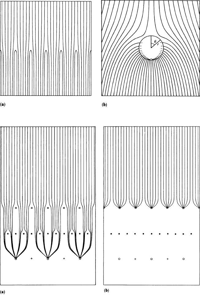
Fig. 3.13a,b Drift field lines in a standard case
(z
1
= 4mm, z
2
= 8mm, z
3
= 12mm, s
1
= 4mm, s
2
= 1mm, s
3
= 2mm). The field lines
between the sense wires and the other electrodes have been omitted for clariy. Squares: gating
grid; black circles: zero-grid; open circles: sense wires; crosses: field wires, (a) gating grid open
(maximal transparency), (b) gating grid closed
3.3 An Ion Gate in the Drift Space 117
V
p
−V
z
V
g
−V
z
=
1
ε
0
⎛
⎝
z
p
−z
2
z
3
−z
2
z
3
−z
2
(z
3
−z
2
) −
s
3
2
π
ln
2
π
r
g
s
3
⎞
⎠
σ
p
σ
g
(3.52)
and
σ
p
σ
g
= K
⎛
⎝
z
3
−z
2
−
s
3
2
π
ln
2
π
r
g
s
3
−(z
3
−z
2
)
−(z
3
−z
2
) z
p
−z
2
⎞
⎠
V
p
−V
z
V
g
−V
z
, (3.53)
where
K =
ε
0
(z
p
−z
2
)
z
3
−z
2
−
s
3
2
π
ln
2
π
r
g
s
3
−(z
3
−z
2
)
2
and V
g
is the potential of the gating grid. In the following we neglect the second
term in the denominator of the factor K, since z
p
−z
2
z
3
−z
2
in the standard case.
Using (3.51) and (3.53) we can calculate the minimum value of V
g
needed for the
full transparency of the gating grid:
V
g
−V
z
≤
4
π
r
g
s
3
V
p
−V
z
z
p
−z
2
z
3
−z
2
−
s
3
2
π
ln
2
π
r
g
s
3
+
z
3
−z
2
z
p
−z
2
(V
p
−V
z
). (3.54)
The second term of (3.54) is the potential difference that makes
σ
g
= 0. The first
term is the additional difference needed to eliminate the positive charges from the
gating grid. In a standard configuration the two terms are comparable.
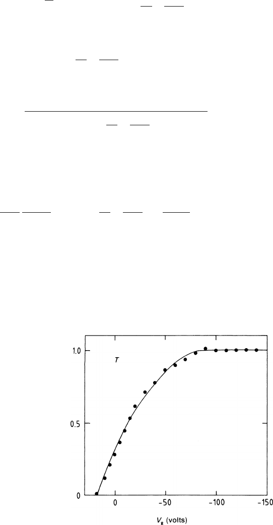
In Fig. 3.14 we compare the transparency calculated according to (3.46–3.53)
for our standard case with measurements performed on a model of the ALEPH TPC
[AME 85-1]. There is good agreement between theory and experiment.
Fig. 3.14 Electron
transparency of a grid with
pitch 2 mm, as a function of
the common potential V
g
applied to the wires. The
electrode configuration
corresponds to Fig. 3.6. The
points represent
measurements by
[AME 85-1]. The line is a
function calculated using
(3.46–3.54)

118 3 Electrostatics of Tubes, Wire Grids and Field Cages
3.3.2 Setting of the Gating Grid Potential with Respect
to the Zero-Grid Potential
In Sect. 3.4 it was shown that because of the high field in the amplification region
the average potential at the position of the zero-grid does not coincide with V
z
.The
potential in the drift region, where the gating grid has to be placed, is given by (3.45).
This formula can be extrapolated at z = z
2
:
V(z
2
)=V
z
+
s
2
2
πε
0
σ
z
ln
2
π
r
z
s
2
, (3.55)
giving the effective potential of the zero-grid seen from the region where the gating
grid has to be placed.
In Sect. 3.3.1 we calculated the condition of full transparency, approximating the
zero-grid as a solid plane at a potential V
z
and referring to it the potential of the
gating grid. In the real case V
g
has to be referred to the effective potential V (z
2
)
given by (3.55).
From what has been shown so far one can deduce that by making V
g
sufficiently
positive all drift field lines terminate on the gating grid and the transparency T is 0.
Figure 3.13a,bb shows how the drift field lines terminate on the gating grid.
3.4 Field Cages
The electric field in the drift region has to be as uniform as possible and ideally
similar to that of an infinitely large parallel-plate capacitor. The ideal boundary con-
dition on the field cage is then a linear potential varying from the potential of the
high-voltage membrane to the effective potential of the zero-grid.
This boundary condition can be constructed, in principle, by covering the field
cage with a high-resistivity uniform material. A very good approximation can be
obtained covering the inner surface of the field cage with a regular set of conducting
strips perpendicular to the electric field, with a constant potential difference
Δ
V
between two adjacent strips:
Δ
V = E
Δ
,
where
Δ
is the pitch of the electrode system.
The exact form of the electric field produced by this system of electrodes can
be calculated with conformal mapping taking advantage of the symmetry of the
boundary conditions [DUR 64]. Figure 3.15 shows the electric field lines and the
equipotentials near the strips in a particular case when the distance between two
strips is 1/10 of the strip width. The electric field very near to the strips is not uni-
form and there are also field lines that go from one strip to the adjacent one. The
transverse component essentially decays as exp(−2
π
t/
Δ
) where t is the distance
from the field cage (see Sect. 3.2), and when t =
Δ
the ratio between the transverse
and the main component of the electric field is about 10
−3
. At larger distances it
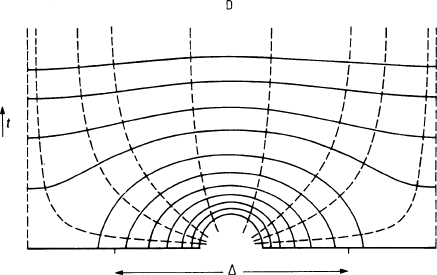
3.4 Field Cages 119
Fig. 3.15 Electric field configuration near the strips of a field cage. Equipotential lines (broken)
and electric field lines (full) are shown. D: drift space;
Δ
: electrode pitch; t: coordinate in the drift
space
becomes completely negligible, showing that this geometry of the electrodes is in-
deed a good approximation of the ideal case. However, the insulators present some
problems.
3.4.1 The Difficulty of Free Dielectric Surfaces
The Dirichlet boundary conditions of the electrostatic problem to be solved in some
volume require the specification of a potential at every point of a closed boundary
surface. When conducting strips are involved that are at increasing potentials, insu-
lators between them are unavoidable, and the potential on these cannot be specified.
If the amount of free charge deposited on these surfaces were known everywhere,
one would have mixed boundary conditions, partly Dirichlet, partly Neumann, and a
solution could be found. In high-voltage field cages there is always some gas ioniza-
tion, and the amount of free charges ready to deposit on some insulator is infinitely
large. How can this uncertainty in the definition of the drift field be limited? There
are several solutions to this difficulty:
Controlled (small, surface or volume) conductivity of the insulator: For every
rate of deposit of ions there is some value of conductivity allowing the transport
of these ions sufficiently fast to the next electrode, so that their disturbing effect is
limited.
Retracted insulator surfaces: If the electrodes have the form indicated in
Fig. 3.16a,ba or b, any field E that may develop at the bottom of the ditch be-
tween conductors owing to charge deposit will be damped by a factor of the order of
exp(−
π
d/s) at the edge of the drift space. (For details of this electrostatic problem,
see e.g. [JAC 75, p. 72.]) A maximum field E is given by the breakdown strength of
the particular gas.
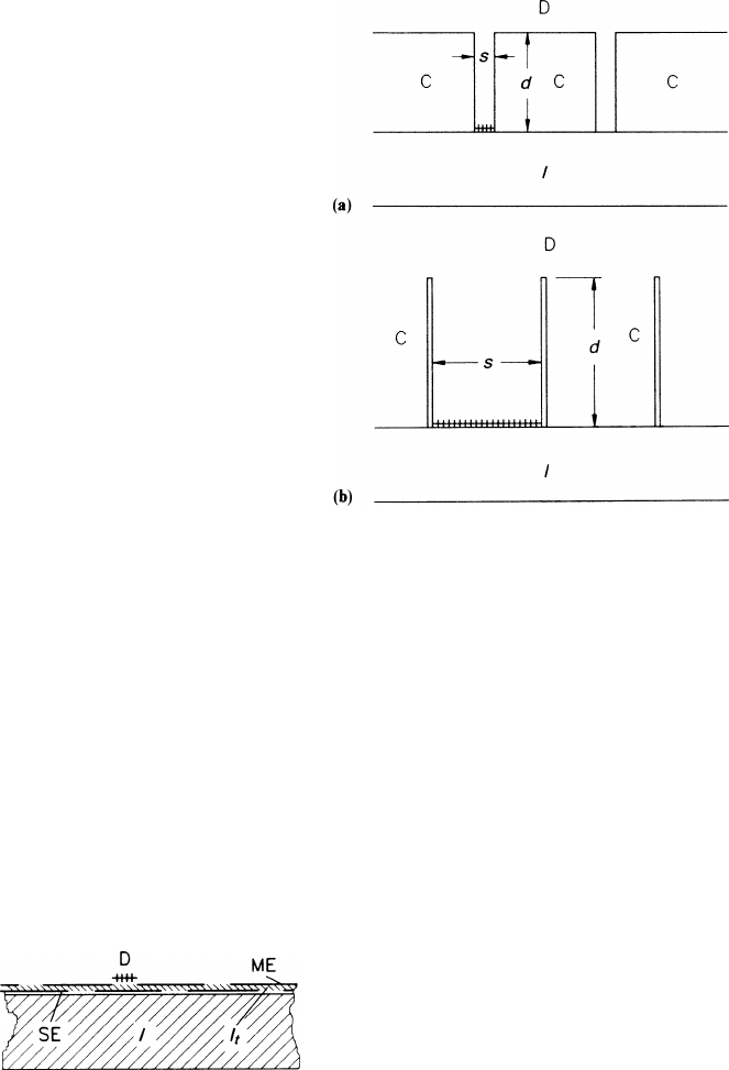
120 3 Electrostatics of Tubes, Wire Grids and Field Cages
Fig. 3.16a,b Field-cage
electrode configuration with
retracted insulator surfaces.
I: insulator, C: conductor, D:
drift space, (a) small gap, (b)
large gap
Thin insulator with shielding electrodes covering the gap from behind: Apart
from the system of main electrodes, there is another set separated by a thin layer of
insulator, and staggered by a half-step according to Fig. 3.17. The purpose of these
shielding electrodes at intermediate potentials is to regularize the field in the drift
region, but also to produce virtual mirror charges of any free charges that may have
deposited in the gap, thus reducing their effect in the drift space.
If we assume that by one of the measures described above the adverse effects
of any charge deposit are sufficiently reduced, we may imagine a smooth (linear)
transition of potential between neighbouring electrodes, and the exact form of the
electric field produced by the system of electrodes at increasing potentials can be
calculated as discussed at the beginning of this section.
Electrostatic distortions were studied by Iwasaki et al. [IWA 83].
Fig. 3.17 Field-cage electrode configuration with secondary electrode strips (SE) covering the
gaps between the main electrode strips (ME) behind a thin insulator foil (It). D: drift space; I:
insulator
3.4 Field Cages 121
3.4.2 Irregularities in the Field Cage
In this subsection we present some studies that have arisen in practice when estimat-
ing the tolerances that had to be respected in the ALEPH TPC for the conductivity
of the insulator, for the match of the gating grid and for the resistors in the potential
divider. We quote the three relevant electrostatic solutions as examples of similar
problems in chambers with different geometry.
If all the electrodes of the field cage are set at the correct potential, the drift field
is uniform and parallel to the axis of the TPC in the whole drift volume. A wrong
setting of the potentials produces a transverse component of the electric field and
causes a distortion of the trajectories of the drifting electrons. In order to study this
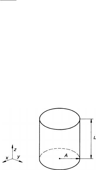
effect in detail the drift volume of the TPC is schematized as a cylinder of length L
and radius A (see Fig. 3.18). The potentials defined on the surface of the cylinder
define the boundary conditions of the electrostatic problem and the drift field inside
the volume. If the potentials on the boundary do not vary with
φ
, the electric field
can only have a transverse component in the radial direction.
In the absence of magnetic field the electrons drift along the electric field line; an
electron placed at the position (r
0
, z
0
) reaches the end of the drift volume at a radial
position
r = r
0
+
0
z
0
E
r
(r,z)
E
z
dz.
The radial component of the field can be calculated solving the Poisson equation in
cylindrical coordinates [JAC 75, p. 108]. Since the ideal setting of the potential does
not produce radial electric field components it is convenient to use as a boundary
condition the difference between the actual and the ideal potentials. This is possible
because the Poisson equation is linear in the potential. Although we discuss the ex-
amples in a cylindrical geometry, they apply to other geometries in a similar way.
Non-Linearity in the Resistor Chain. The potential of the strips of the field cage are
defined connecting them to a linear resistor chain. The strips are insulated from the
external ground by an insulator that has a finite resistivity and that is in parallel with
the resistors of the chain. It can be shown that the resistance to ground of a strip
placed at a position z is
Fig. 3.18 Scheme of a
cylindrical TPC drift region
122 3 Electrostatics of Tubes, Wire Grids and Field Cages
R(z)=R
tot
z
L
−
1
6
z
L
3
R
tot
R
man
,
where R
tot
is the resistance of the whole resistor chain and R
man
is the resistance
of the insulator mantel across the wall of the insulator. This non-linear resistance
produces a potential distribution that differs from the linear one by
Δ
V(z)=
Z
L
−
Z
L
3
V
p
R
tot
R
man
R
tot
R
man
1,
where V
p
is the potential of the central electrode. This error potential can be approx-
imated by
Δ
V(z) ≈
0.38
6
V
p
R
tot
R
man
sin
π
z
L
.
Following Jackson’s formalism [JAC 75] it can be shown that the radial displace-
ment of an electron drifting from the point (r, z)is
Δ
r ≈
0.38
6
R
tot
R
man
L
iJ
1
i
π
r
L
J
0
i
π
A
L
cos
π
z
L
−1
,
where J
0
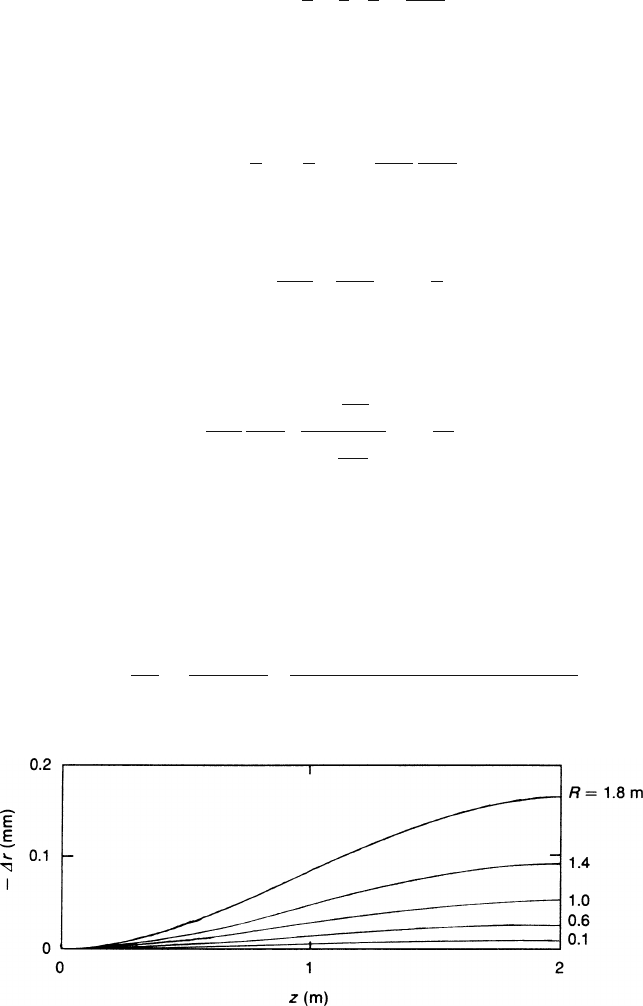
are the Bessel functions of order 0 and 1. Figure 3.19 shows a plot of
Δ
r
as function of z for different values of r assuming L = A = 2m and R
tot
/R
man
= 10
−3
.
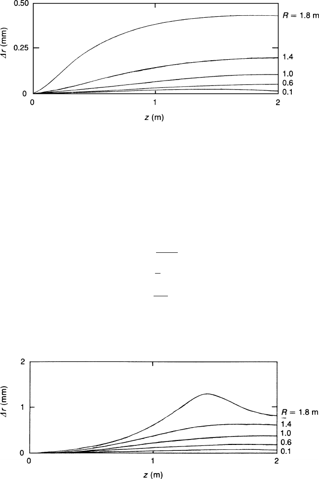
Mismatch of the Gating Grid. The potentials of the field cage have to match that of
the last wire plane as discussed in Sect. 3.2. An error
Δ
V in the potential of the last
electrode of the field cage produces a radial displacement
Δ
r = 2L
Δ
V
V
p
∑
n
J
1
(x
n
r/A)
J
1
(x
n
)x
n
cosh[
π
(L −z)(x
n
/A) −cosh(Lx
n
/A)
sinh(Lx
n/A
)
,
Fig. 3.19 Radial displacement r of the arrival point of an electron, caused by a resistance R
man
of
the insulator mantle a thousand times the value of the resistor chain,
Δ
r is shown as a function of
the starting point z, R in the example A = L = 2m
3.4 Field Cages 123
Fig. 3.20 Radial displacement
Δ
r of the arrival point of an electron, caused by a voltage mismatch
Δ
V between the last electrode of the field cage and the last wire plane, amounting to ΔV/V
p
= 10
−4
of the drift voltage.
Δ
r is shown as a function of the starting point (z, R) in the example A = L = 2m
where x
n
= k
n
A and J
0
(k
n
)=0.
Figure 3.20 shows a plot of
Δ
r as a function of z for different values of r assuming
L = A = 2m and
Δ
V/V
p
= 10
−4
.
Resistor Chain Containing One Wrong Resistor. If in the voltage-divider chain one
of the resistors (placed at z = ¯z) has a wrong value, it induces an error in the potential
of the field cage:
Δ
V(z)=
−
Δ
V
L
z, z < ¯z,
Δ
V
1−
z
L
, z > ¯z,
Δ
V = V
p
Δ
R
R
tot
,
where
Δ
R is the error in the resistance of that particular resistor and R
tot
is the total
resistance of the chain. The induced radial displacement is
Fig. 3.21 Radial displacement
Δ
r of the arrival point of an electron, caused by one wrong resistor
value R
∗
= R +
Δ
R,where
Δ
R/R
tot
= 1/400 of the value of the total resistor chain.
Δ
r is shown as
a function of the starting point (z, R) in the example A = L = 2m

124 3 Electrostatics of Tubes, Wire Grids and Field Cages
Δ
r = L
Δ
R
r
tot
1
π
∑
iJ
1
(in
π
r)/L
J
0
(in
π
A)/L
1
n
cos
n
π
¯z
L
cos
n
π
z
L
−1
.
Figure 3.21 shows a plot of
Δ
r as a function of z for different values of r for a
particular case L = A = 2m, z = 1.4m,
Δ
R/R
tot
= 1/400.
We have computed in this subsection three specific cases of field-cage prob-
lems in the spirit of showing the order of magnitude of the relevant electron
displacements. The design of the drift chamber must be such that the displace-
ment
Δ
r induced by such irregularities remains small in comparison to the required
accuracy.
References
[ABR 65] M. Abramowitz and I.A. Stegun, Handbook of Mathematical Functions, (Dover,
New York 1965) p. 75
[AME 85-1] S.R. Amendolia et al., Influence of the magnet field on the gating of a time projection
chamber, Nucl. Instrum. Methods A 234, 47 (1985)
[DUR 64] Durand, Electrostatique vol. II (Masson et C. edts., Paris 1964)
[FAB 04] C.W. Fabjan and W. Riegler, Trends and Highlights of VCI 2004, Nucl. Instr. Meth.
Phys. Res. A 535, p. 79-87 (2004)
[IWA 83] H. Iwasaki, R.J. Maderas, D.R. Nygren, G.T. Przybylski, and R.R. Sauerwein,
Studies of electrostatic distortions with a small time projection chamber, in The Time
Projection Chamber (A.I.P. Conference Proceedings No. 10 TRIUMF, Vancouver,
Canada, 1983)
[JAC 75] J.D. Jackson, Classical Electrodynamics (Wiley, New York 1975)
[MOR 53] P.M. Morse and H. Feshbach, Methods of Theoretical Physics (McGraw Hill,
New York 1953).
[PUR 63] E.M. Purcell, Electricity and Magnetism (Berkeley Physics Course Vol. II, McGraw
Hill, New York 1963) Problem 9.11
[VEN 08] R. Veenhof, Drift Chamber Simulation Program Garfield, (1984–2008)
[WEN 58] G. Wendt, Statische Felder und station
¨
are Str
¨
ome in Handbuch der Physik, Vol. XVI
(Springer, Berlin Heidelberg 1958) p. 148

Chapter 4
Amplification of Ionization
4.1 The Proportional Wire
Among all the amplifiers of the feeble energy deposited by a particle on its passage
through matter, the proportional wire is a particularly simple and well-known exam-
ple. When it is coupled with a sensitive electronic amplifier, a few – even single –
electrons from the ionization of a particle can be observed, which create ionization
avalanches in the high electric field near the surface of the thin wire. The develop-
ment of the proportional counter started as long ago as 1948; for an early review,
see [CUR 58]. The proportional counter is also treated in text books on counters in
general, for example those of Korff [KOR 55] and Knoll [KNO 79]. The latter con-
tains a basic list of reference texts. The classical monograph by Raether [RAE 64]
deals with electron avalanches in a broader context.
As an electron drifts towards the wire it travels in an increasing electric field E,
which, in the vicinity of the wire at radius r, is given by the linear charge density
λ
on the wire:
E =
λ
2
πε
0
1
r
.
In the absence of a magnetic field, the path of the electron will be radial. The
presence of a magnetic field modifies the path (as discussed in Chaps. 2 and 7) but,
if the electric field is strong enough, the trajectory terminates in any case on the
wire.
Once the electric field near the electron is strong enough so that between colli-
sions with the gas molecules the electron can pick up sufficient energy for ionization,
another electron is created and the avalanche starts. At normal gas density the mean
free path between two collisions is of the order of microns; hence the field that starts
the avalanche is of the order of several 10
4
V/cm, and the wire has to be thin, say a
few 10
−3
cm, for 1 or 2 kV.
As the number of electrons multiplies in successive generations (Fig. 4.1), the
avalanche continues to grow until all the electrons are collected on the wire. The
avalanche does not, in general, surround the wire but develops preferentially on
the approach side of the initiating electrons (cf. Sect. 4.3). The whole process
W. Blum et al., Particle Detection with Drift Chambers, 125
doi: 10.1007/978-3-540-76684-1
4,
c
Springer-Verlag Berlin Heidelberg 2008