Blum W., Riegler W., Rolandi L. Particle Detection with Drift Chambers

Подождите немного. Документ загружается.

76 2 The Drift of Electrons and Ions in Gases

Modern developments may be followed in the Proceedings of the International

Conference on the Physics of Electronic and Atomic Collisions, see especially

[CHR 81]. One distinguishes two-body and three-body processes.

The two-body process involves a molecule M that may or may not disintegrate

into various constituents A, B, ..., one of which forms a negative ion:

−

+ M → M

−

+ M → A

−

+ B + ...

The break-up of the molecule owing to the attaching electron is quite common and

is called dissociative attachment. The probability of the molecule staying intact is

generally higher at lower electron energies. The rate R of attachment is given by the

cross-section

, the electron velocity c, and the density N of the attaching molecule:

R = c

N = kN. (2.76)

The rate is proportional to the density. The constant of proportionality is called

the two-body attachment rate-constant k.

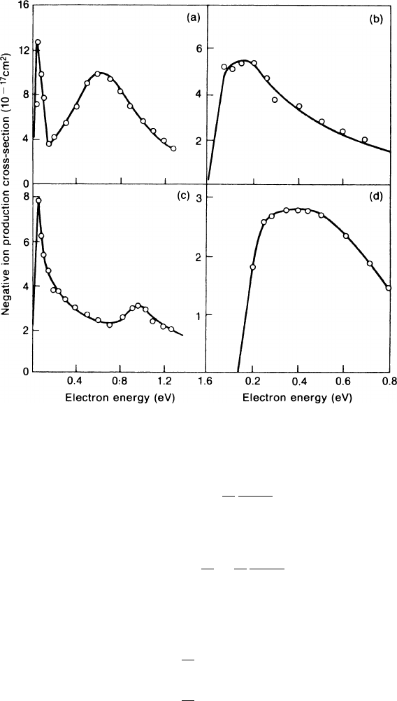
As examples of strong attachment of slow electrons, we depict in Fig. 2.12a-d

the measured cross-sections of some freons. The rate constants of many other

halogen-containing compounds are known [MCC 81]; some of them reach several

−8

−1

at low (thermal) electron energies.

Among the three-body processes, the Bloch–Bradbury process is the best known

[BLO 35, HER 69]. It plays an important role in the absorption of electrons by

oxygen molecules. At energies below 1 eV, the electron is attached to the oxygen

molecule that forms the excited and unstable state O

∗−

. Unless the energy of excita-

tion is carried away by a third body X during the lifetime of the excitation, the O

∗−

ion will lose its electron, which is then no longer attached. The lifetime

is of the

order of 10

−10

s; experimental determinations span the range between 0.02×10

−10

and 1.0 ×10

−10

s, and theoretical calculations come out between 0.88×10

−10

and

3 ×10

−10

s [HAT 81]. The rate R of effective attachment depends on

,aswellas

on the two collision rates and the cross-sections for the two processes,

−

+ O

→ O

∗−

+ X → O

∗−

+ X.

Let us look at a swarm of electrons in a gas that contains O

molecules with

density N(O

) and third bodies X with density N(X). Per electron, let the rate dn/dt

of formation of the O

∗−

state be 1/T

; if the rate of spontaneous decay is n/

and the

rate of de-excitation through collision with third bodies n/T

, then the equilibrium

number n per electron of O

∗−

states is given by

2.2 The Microscopic Picture 77

Fig. 2.12a-d Cross-sections for the production of negative ions by slow electrons in (a) CCl

(b) CCl

, (c) CF

Iand(d) BCl

, observed by Buchel’nikova [BUC 58]

n =

+ T

Therefore, the rate R of effective attachment of one electron is

R =

+ T

The rates 1/T

and 1/T

may be expressed by the cross-sections a and relative

velocities c:

= c

N(O

= c

N(X).

In our application, c

is the instantaneous electron velocity and c

the velocity of

the thermal motion between the molecules O

and X.

78 2 The Drift of Electrons and Ions in Gases

For ordinary pressure and temperature we have T



, and therefore the rate is

given by

R =

N(O

)N(X)=k

N(O

)N(X). (2.77)

It is proportional to the product of the two densities. The three-body attachment

coefﬁcient k depends on the electron energy through c

and

, on the temperature

through c

, and on the nature of the third body through

. The rate varies linearly

with each concentration and quadratically with the total gas density.

In the 1980’s another three-body process has been identiﬁed as making an impor-

tant contribution to the absorption of electrons on O

molecules. The O

molecules

and some other molecules X form unstable van der Waals molecules:

+ X ↔ (O

X).

These disintegrate if hit by an electron, which ﬁnally remains attached to the O

molecule:

−

+(O

X) → O

−

+ X.

Since the concentration of van der Waals molecules in the gas is proportional to

the product N(O

)N(X), the dependence on pressure and concentration ratios in a

ﬁrst approximation is the same as in the Bloch–Bradbury process.

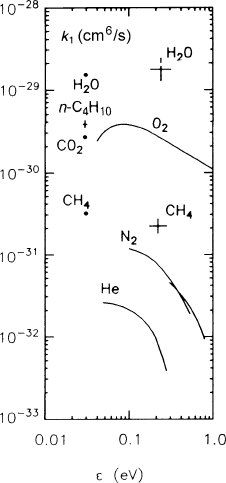
The relative importance of these two three-body attachment processes has been

measured with the help of an oxygen-isotope effect [SHI 84]. The authors ﬁnd

Fig. 2.13 Some three-body

attachment coefﬁcients for

quoted from Massey

et al. [MAS 69]. The two

crosses are measurements

by Huk et al. [HUK 88]; for

the hydrocarbons at thermal

energy, see [SHI 84]

2.3 Results from the Complete Microscopic Theory 79

examples where the van der Waal mechanism dominates, whilst the Bloch–Bradbury

process is weak; also at higher gas pressures, the van der Waals mechanism makes

a strong contribution.

For the operation of drift chambers, the absorption of electrons is a disturbing

side effect that can be avoided by using clean gases. Therefore we leave out further

reﬁnements that are discussed in the literature.

Some measured three-body attachment coefﬁcients for O

are shown in Fig. 2.13

as functions of the electron energy. It can be seen that the H

O molecule is much

more effective as the third body than the more inert atoms or the nitrogen molecule.

The three-body O

attachment coefﬁcient involving the methane molecule is

large enough to cause electron losses in chambers where methane is a quenching

gas. For example (compare Table 11.4), with 20% CH

at 8.5 bar, an oxygen con-

tamination of 1 ppm will cause an absorption rate of 2000/s, or roughly 3%/m of

drift at a velocity of 6cm/μs. More information on electron attachment is collected

in Chap. 12.

2.3 Results from the Complete Microscopic Theory

In this section we quote without proof results for mobility and diffusion in the

framework of the complete microscopic theory. The reader is referred to Huxley

and Crompton [HUX 74] and to Allis [ALL 56] for a more detailed discussion.

2.3.1 Distribution Function of Velocities

The principal approximation of Sect. 2.2 was to take a single velocity c to represent

the motion between collisions of the drifting electrons. In reality, these velocities

are distributed around a mean value according to a distribution function

(c)dc,

which represents the isotropic probability density of ﬁnding the electron in the three-

dimensional velocity interval dc

at c. Therefore the distribution function is

normalized so that

∞



(c)dc = 1.

The term ‘isotropic’ actually refers to the ﬁrst, isotropic, term of an expansion in

Legendre functions of the probability distribution for the vector c.

The shape of the distribution depends on the way in which the energy loss and

the cross-section vary with the collision velocity. The regime of elastic scattering

as well as a good part of the regime of inelastic scattering can be described by two

80 2 The Drift of Electrons and Ions in Gases

functions: an effective cross-section

(c), and the fractional energy loss λ(c)(

(c)

is sometimes called the momentum transfer cross-section). Electron drift velocities

that are appropriate for drift chambers are achieved by electric ﬁelds that are high

enough to make the random energy of the electron much higher than the thermal

energy of the gas molecules. Therefore we may neglect thermal motion. Absorption

or production of electrons (ionization) is equally excluded.

With these assumptions the distribution of the random velocities can be derived in

the framework of the Maxwell–Boltzmann transport equations [HUX 74, SCH 86,

ALL 56]:

(c)=const exp

⎡

⎣

−3



⎤

⎦

= const exp

⎡

⎣

−3m



⎤

⎦

, (2.78)

where

= mc

/2, and

= eEl

= eE/(N

) is the energy gained through a mean

free path l

in the direction of the ﬁeld. The distribution function can also be written

as an integral over the collision frequency

= cN

. The second form of (2.78)

lends itself to the generalization owing to the presence of a magnetic ﬁeld. For a

discussion of the range of validity of our assumptions, the reader is also referred to

the quoted literature.

In order to make a picture of such velocity distributions, we consider two limit-

ing cases.

• If both the collision time

and the fractional energy loss are independent of c,

then f

(

√

)

exp



−







, (2.79)

with

3λ





• If both the mean free path l

= c

and the fractional energy loss are independent

of c – an approximation that is sometimes useful in a limited range of energies –

then f

πΓ

(3/4)

exp



−







, (2.80)

with

3λ





Once f

averages over all velocities c.

2.3 Results from the Complete Microscopic Theory 81

Fig. 2.14 Normalized

Maxwell and Dryvesteyn

distributions according to

(2.79) and (2.80). The proba-

bility density is given in units

of c/

. The r.m.s. values are

indicated

2.3.2 Drift

The drift velocity is given by

u =

∞



(c)



(c)



dc = −

∞



(c)

(c)dc. (2.81)

The two expressions are related to each other by a partial integration and by the

fact that the mean collision frequency

(c)c. The drift velocity depends on

E and N only through the ratio E/N.

Another way of writing (2.81) is to use brackets for denoting the average over

the velocity distribution. With a little algebra, we obtain

u =



+





E. (2.82)

This shows that expression (2.14) is recovered not only in the obvious case that

is independent of c, but already when only the average cd

/dc vanishes.

In the case of a constant

and λ, using the Druyvesteyn distribution (2.80), we

may derive the mean square random velocity c

and the square of the drift velocity

from (2.81). We ﬁnd that

c

 =



0.854,



0.855.

82 2 The Drift of Electrons and Ions in Gases

A comparison with (2.19) and (2.20) shows that there are extra factors of 0.854

and 0.855 resulting from the ﬁnite width of the velocity distribution.

2.3.3 Inclusion of Magnetic Field

In Sect. 2.2.3 we have seen that the addition of a magnetic ﬁeld to electrons drift-

ing in an electric ﬁeld will change their effective random velocity c unless the two

ﬁelds are parallel, so there has to be a change in the distribution function. Following

Allis and Allen [ALL 37] (but see also [MAS 69, HUX 74]), we quote the result for

the case where the two ﬁelds are orthogonal to each other. The distribution takes

the form

(c)=const exp

⎡

⎣

−



λ(

)[

(

⎤

⎦

, (2.83)

where the cyclotron frequency

=(e/m)B is, of course, independent of

This function depends on two constants of nature e and m, on two functions of

the electron energy

(

) and λ(

), and on three numbers (E, B, N) in the hands of

the experimenter, of which two (say E/N and B/N) are independent. For arbitrary

orientation of the ﬁelds, f

would depend on the angle between the two ﬁelds.

In the presence of a magnetic ﬁeld, the drift-velocity vector depends on both

the electric and magnetic ﬁelds. The corresponding mobility tensor is

, so that

(summation over common indices is understood). The three diagonal

components and the six off-diagonal terms are given by the following expressions:

= −

∞



(

)

(

)

(c)dc,

= −

∞



(

νε

ik j

)

(

)

(c)dc.

(2.84)

where the fully antisymmetric symbol

ik j

represents a sign-factor that is equal to

+1 for all even permutations of 123, to −1 for all odd ones, and to zero if any two

elements are equal;

, are the components of the magnetic ﬁeld, multiplied

by e/m,

; f

for the two ﬁelds. As in the case of the scalar mobility, if

is independent of c then

one recovers the expression (2.5) derived from the equation of motion with friction.

Deviations from this relation can therefore be expected to the extent that

varies

with c. See also the discussion in Sect. 2.4.5.

We notice that the number density N of gas molecules is a scaling factor, not only

for the electric ﬁeld but also for the magnetic ﬁeld. If in (2.84) we divide numerator

and denominator by

=(e/m)

, then all terms containing

’s appear either as

or as

= N

2.4 Applications 83

The dependence of the drift-velocity vector on the three scalar quantities E, B,

and N may therefore be written in the form





, (2.85)

where

is the angle between the ﬁelds.

This relation is important when it comes to a discussion of the gas pressure in

drift chambers (Chap. 12).

2.3.4 Diffusion

As given in the quoted literature, the isotropic diffusion coefﬁcient is derived from

the velocity distribution function through the integral

D = 4

∞



(c)

(c)c

dc. (2.86)

We note that expression (2.61) represented the case of one unique velocity,

(c)=

(c −c).

The magnetic anisotropy caused by a B ﬁeld may be described by the 3×3 tensor

. Its elements are given by

∞



(

)

(

)

(c)c

dc,

∞



(

νε

ik j

)

(

)

(c)c

dc.

(2.87)

For the electric anisotropy of diffusion, we must retain in the velocity distribution

its dependence on position; the reader is referred to the literature [PAR 69].

2.4 Applications

In this section we discuss few practical applications of the formulae derived in the

previous sections.

2.4.1 Determination of

(

) and λ(

) from Drift Measurement

In the drift of ions and electrons in gases, the quantities that are important for track

localization are the drift velocity and the diffusion tensor. In this chapter we have

84 2 The Drift of Electrons and Ions in Gases

described how they are derived as functions of E and B from the two functions of

the collision velocity,

fraction of energy loss per collision. However, these two functions are generally

not known from independent measurements, and one goes in the opposite direction:

starting from measurements of u(E) and D(E)/

(E), one tries to ﬁnd, with some

intuition,

the formulae described in Sect. 2.3. If the measured values coincide with the ones

“recalculated” from the guessed

applied to electrons in argon by Frost and Phelps in 1964 [FRO 64].

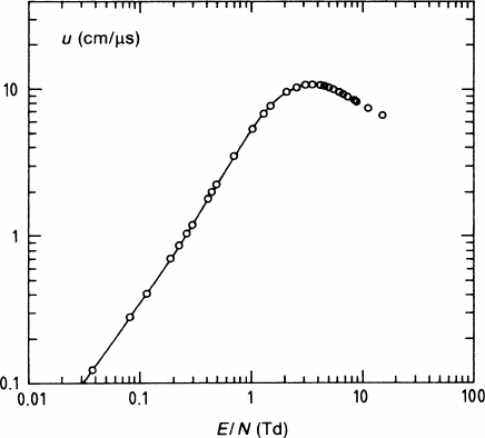
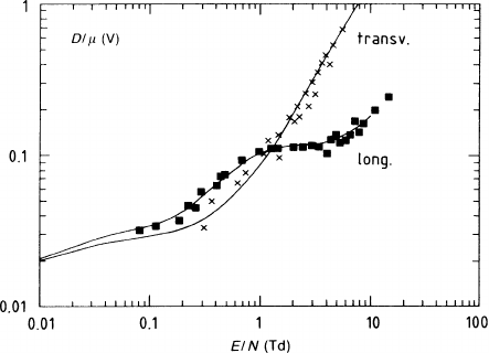
In the work of B. Schmidt [SCH 86], considerable progress is visible not only in

the accuracy of his measurements – which is near 1% in the drift velocity and 5%

in D/

– but also in the inclusion of the electric anisotropy of diffusion. He studied

the noble gases and some molecular gases–chieﬂy methane–which are useful in drift

chambers. In Fig. 2.15 we see the CH

drift-velocity measurements, and in Fig. 2.16

the measurements of the transverse and longitudinal diffusion. Superimposed we

ﬁnd curves that represent the recalculated values. The effective (momentum trans-

fer) cross-section of methane and the energy loss factor of methane used in their

calculation have already been shown in Figs. 2.2a and 2.2b as functions of the

electron energy. The consistency of these results leaves no doubt that the method

is correct, although the assessment of the errors to

(

) and λ(

) remains difﬁ-

cult. It is possible to give λ(

) a form that is consistent with plausible assumptions

about the quadrupole moments of the methane molecule. Similar computations were

done by Biagi [BIA 89]. A special case concerning water contamination is treated

in Sect. 12.3.3.

Fig. 2.15 Measured and recalculated electron drift velocity in CH

as a function of the reduced

electric ﬁeld. One Townsend (Td) equals 10

−17

Vcm

.[SCH 86]

2.4 Applications 85

Fig. 2.16 Measured and recalculated transverse and longitudinal electron diffusion in CH

[SCH 86]. The ratio of the diffusion coefﬁcients over the mobility is shown as a function of the

reduced electric ﬁeld

There are microwave relaxation measurements that allow an alternative deriva-

tion of the cross-sections of some gases; also, there are quantum-mechanical cal-

culations for the noble gases. Where a comparison of cross-sections can be made,

they are identical within factors of 2 to 5, and often much better. According to the

calculations, the minimum is sharper than that derived from the drift measurement

because the wide energy distribution smears it out. For more details, the reader is

referred to the literature.

There is a very large number of measurements of electron drift velocities and

diffusion coefﬁcients. Many of them are collected in two compilations [FEH 83]

and [PEI 84], which also contain other material that is of interest with respect to

drift chambers.

Measurements in magnetic ﬁelds are rare; we present some examples in

Sect. 2.4.7. Precision reproductions of magnetic data, and determinations of

(

)

and λ(

) from them, have not yet been done.

2.4.2 Example: Argon–Methane Mixture

In this subsection we want to collect and interpret some drift and diffusion measure-

ments for argon + methane mixtures without magnetic ﬁeld. This gas has been

investigated more systematically than most others, and is being used in several

large TPCs.

The measurements, done by Jean-Marie et al. [JEA 77], of the drift velocity as

a function of the electric ﬁeld E at atmospheric pressure are presented in Fig. 2.17.

For all mixing ratios R there is a rising part at low E and a falling part at high E.The

maxima occur at values E

, which depend almost linearly on the CH

concentration,