Blank L., Tarquin A. Engineering Economy (McGraw-Hill Series in Industrial Engineering and Management)
Подождите немного. Документ загружается.

SECTION 19.4
Expected Value and Standard Deviation
TABLE
19-3
Computation
of
Standard
Deviation
Using
~qua
tion [19.11]
withX
=
$116.29, Example 19.6
x
(X-
X)
(X
-
X)2
$ 40
-76.29
5,820.16
66
-50.29
2,529.08
75
-41.29
1,704.86
92
- 24.29
590.00
107
- 9.29
86.30
159
+42.71
1,824.14
275
+158
.71
25,188.86
--
$814 $37,743.40
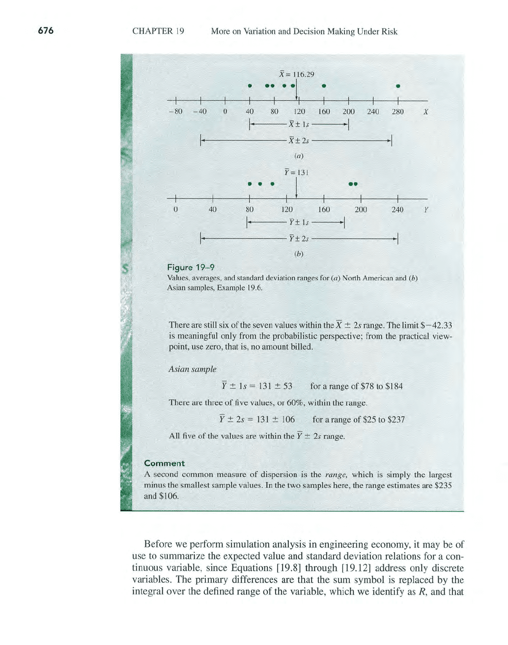
TABLE
19-4
. Computation
of
Standard
Deviation
Using Equa-
tion [19.
12]
with Y =
$131, Example 19.6
y
y2
$ 84
7,056
90
8,100
104
10,816
187
34,969
190
36,100
$655
97,041
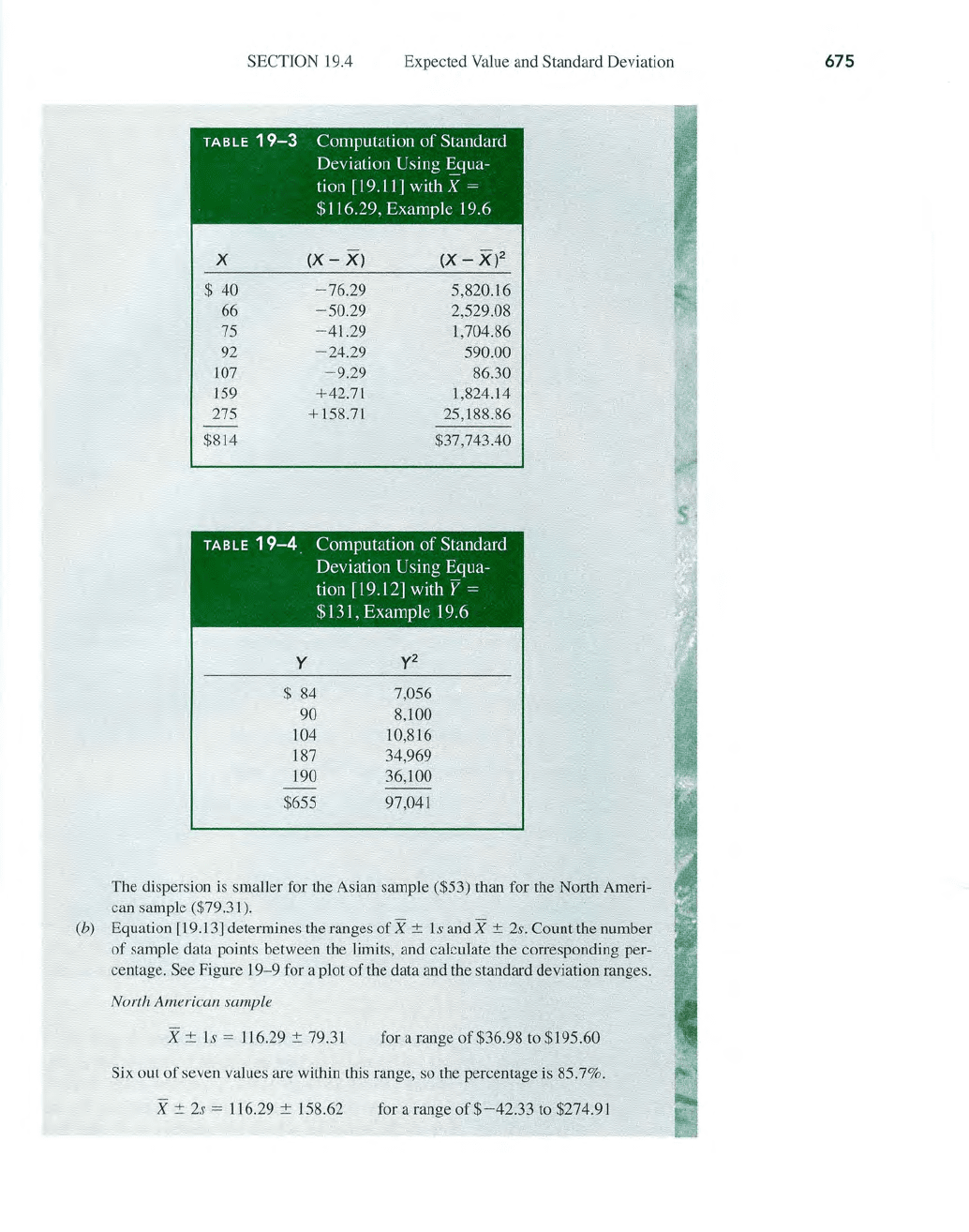
The dispersion is smaller for the Asian sample ($53) than for the North Ameri-
can sample ($79.31).
(b) Equation [19.13] determines the ranges
of
X
:!:
Is
and X
:!:
2s.
Count the number
of
sample data points between the limits, and calculate the corresponding per-
centage.
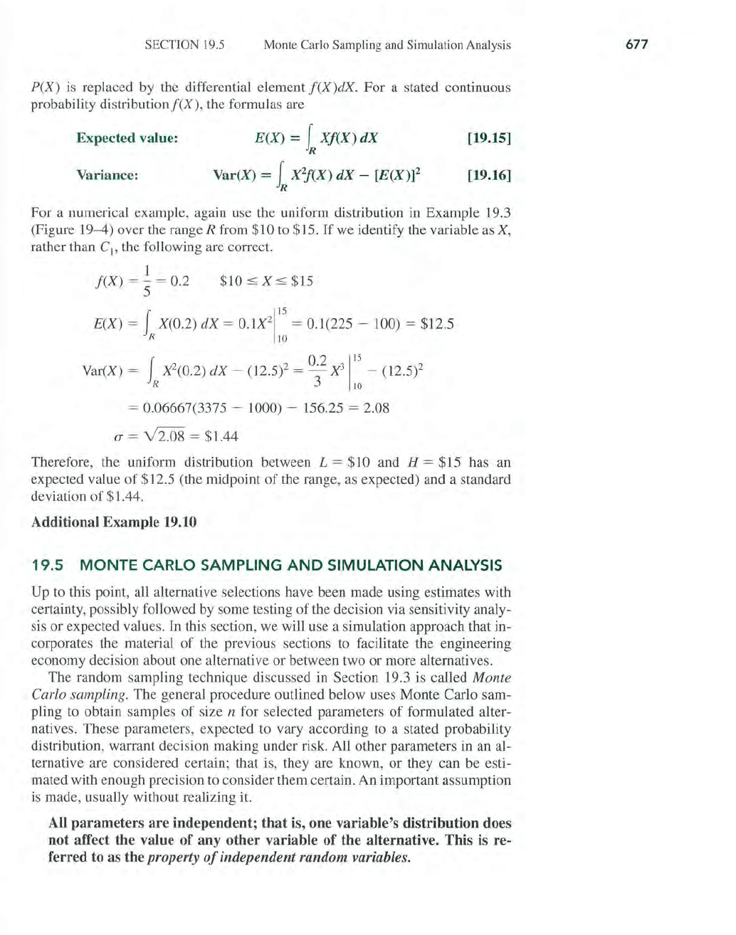
See Figure
19
- 9 for a plot
of
the data and the standard deviation ranges.
North American sample
X
:!:
Is = 116.29
:!:
79.31
for a range
of
$36.98 to $195.60
Six out
of
seven values are within this range, so the percentage is 85.7%.
X:!:
2s
= 116.29 :!: 158.62
for a range
of
$-42.33
to $274.91
675
676
CHAPTER
19
More on Variation and Decision Making Under Risk
x=
116.29
•
••
· ·1
•
•
I I
- 80
- 40
0
40
80
12
0
160
200 240
280
X
I·
X±
Is
·1
I·
X±2s
·1
(a)
y=
131
• •
•
1
••
I
0
40
80
120
160
200 240
Y
I·
Y±
Is
·1
I·
Y±2s
·1
(b)
Figure
19-9
Values, averages, and standard deviation ranges for (a) North American and (b)
Asian samples, Example 19.
6.
There are still six
of
the seven values within the X ± 2s range. The limit $- 42.33
is meaningful only from the probabilistic perspective; from the practical view-
point, use zero, that is, no amount billed.
Asian sample
Y ±
Is
=
131
± 53
for a range
of
$78 to $184
There are three
of
five values, or 60%, within the range.
Y ± 2s =
131
± 106
for a range
of
$25 to $237
All five
of
the values are within the Y ± 2s range.
C9mment
A second common measure
of
dispersion is the range, which is simply the largest
minus the smallest sample values.
In the two samples here, the range estimates are $235
and $106.
Before we perform simulation analysis in engineering economy, it may be
of
use
to
summarize the expected value and standard deviation relations for a con-
tinuous variable, since Equations [19.8] through [19.
12]
address only discrete
variables. The primary differences are that the sum symbol is replaced by
th
e
integral over the defined range
of
the variable, which we identify
as
R,
and that
SECTION 19.5 Monte Carlo Sampling and Simulation Analysis
P(X) is replaced by the differential element
f(X)dX.
For
a stated continuous
probability distributionf(X), the formulas are
Expected value:
E(X)
= L
Xf(X)
dX
R
[19.15]
Var(X)
= L
X'l(X)
dX
- [E(X)]2
R
Variance: [19.16]
For a numerical example, again use the uniform distribution in Example 19.3
(Figure 19- 4) over the range
R from $10 to $15.
If
we identify the variable as X,
rather than C
1
, the following are correct.
f(X)
=
~
=
02
5 .
$10::;
X::;
$15
E(X)
= f X(0.2)
dX
=
0.IX2115
= 0.1(225 - 100) = $12.5
R
10
Var(X) = f X2(0.2)
dX
-
(l2.5f
= 0.2
X3115
- (12.5)2
R 3
10
= 0.06667(3375 - 1000) - 156.25 = 2.08
(J
=
Y2
.08 = $1.44
Therefore, the uniform distribution between
L = $10 and H = $15 has an
expected value
of
$12.5 (the midpoint
of
the range, as expected) and a standard
deviation
of
$1.44.
Additional Example 19.10
19.5
MONTE
CARLO SAMPLING
AND
SIMULATION ANALYSIS
Up to this point, all alternative selections have been made using estimates with
certainty, possibly followed by some testing
of
the decision via sensitivity analy-
sis or expected values. In this section, we will use a simulation approach that in-
corporates the material
of
the previous sections to facilitate the engineering
economy decision about one alternative
or
between two or more alternatives.
The random sampling technique discussed in Section 19.3 is called
Monte
Carlo sampling. The general procedure outlined below uses Monte Carlo
sam
-
pling to obtain samples
of
size n for selected parameters
of
formulated alter-
natives. These parameters, expected to vary according to a stated probability
distribution, warrant decision making under risk. All other parameters in an al-
ternative are considered certain; that is, they are known,
or
they can be esti-
mated with enough precision to consider them certain. An important assumption
is made, usually without realizing it.
All
parameters
are
independent;
that
is, one variable's distribution does
not
affect the value of any
other
variable of the alternative. This is re-
ferred to as the
property
of
independent
random
variables.
677
678
CHAPTER
19
More on Variation and Decision Making Under Risk
The
simulation approach to engineering
economy
analysis is summarized in
the following
ba
sic steps.
Step
1.
Formulate aJternative(s).
Set
up each alternative in the form to
be
considered using engineering
economic
analysis, and select the mea-
sure
of
worth upon which to base the decision.
Determine
the form
of
the relation(s) to calculate the measure
of
worth.
Step
2. Parameters with variation. Select the parameters in each alterna-
tive to
be
treated as random variables. Estimate values for all other
(certain) parameters for the analysis.
Step
3. Determine probability distributions.
Determine
whether each
variable is discrete
or
continuous, and describe a probability distribu-
tion for each variable in each alternative.
Use
standard distributions
where
possible to simplify the sampling process and to prepare for
computer-based simu lation.
Step 4.
Random sampling. Incorporate the
random
sampling
procedure
of
Section 19.3 (the first
four
steps) into this procedure. This results in
the
cumulative
distribution, assignment
of
RNs, selection
of
the RNs,
and a
sample
of
size n for each variable.
Step 5.
Measure
of
worth calculation.
Compute
n values
of
the
se
lected
measure
of
worth from the relation(s) determined in step I.
Use
the es-
timates made with certainty and the
n
sample
values for the varying
parameters. (This is when the property
of
independent
random
vari-
ables is actually applied.)
Step
6. Measure
of
worth description.
Construct
the probability distribu-
tion
of
the measure
of
worth, using between 10
and
20
cells
of
data,
and calculate measures such as
X, s, X ±
fS
,
and
relevant probabilities.
Step 7.
Conclusions.
Draw
conclusions
about
each alternative, and
decide
which
is
to be selected.
If
the alternative(s) has (have) been previously
evaluated
under
the assumption
of
certainty for all parameters,
com-
parison
of
results may help with the final decision.
Example
19
.7 illustrates this
procedure
using an
abbreviated
manual simula-
tion
ana
lysis, and
Example
19.8 utilizes
spreadsheet
simulation
for the
same
estimates.
Yvonne Ramos
is
the CEO
of
a chain
of
50 fitness centers
in
the United States and
Canada.
An
equipment salesperson has offered Yvonne two long term opportunities on
new aerobic exercise systems, for which the usage
is
charged to customers on a per-use
basis on top
of
the monthly fees paid by customers. As an enticement, the offer includes
a guarantee
of
annual revenue for one
of
the systems for the first 5 years.
Since this
is
an entirely new and risky concept
of
revenue generation, Yvonne wants
to do a careful analysis
of
each alternative. Details for the two systems follow:
System
1. First cost is P = $12,000 for a set period
of
n = 7 years with no salvage
va
lu
e. No guarantee for annual net revenue
is
offered.
SECTION 19.5 Monte Carlo Sampling and Simulation Analysis
System 2. First cost is
P = $8000, there is no salvage value, and there
is
a guar-
anteed annual net revenue
of
$1000 for each
of
the first 5 years, but after this
period, there is
no
guarantee. The equipment with updates may be useful
up
to
15
years, but the exact number is not known. Cancellation anytime after the initial
5 years
is
allowed, with
no
penalty.
For either system, new versions
of
the equipment will be installed with no added costs.
If
a MARR
of
15% per year is required, use PW analysis
to
determine
if
neither, one, or
both
of
the systems should be installed.
Solution
by
Hand
Estimates which Yvonne makes
to
correctly use the simulation analysis procedure are
included in the following steps.
Step
1.
Formulate
alternatives. Using PW analysis, the relations for system 1
and system 2 are developed including the parameters known with certainty.
The symbol NCF identifies the net cash flows (revenues), and NCF
c
is the
guaranteed NCF
of
$1000 for system
2.
PW
j
=
-Pj
+ NCF
j
(P/A,15%,n
j
)
PW
2
=
-P
2
+ NCF
c
(P/A,15%,5)
+ NCF
2
(P/A,15%,n
2
-5)(P/F,15%,5)
[19.17]
[19.18]
Step
2.
Parameters
with variation. Yvonne summarizes the parameters esti-
mated with certainty and makes distribution assumptions about three param-
eters treated as random variables.
System 1
Certainty. P
j
= $12,000;
nj
= 7 years.
Variable. NCF
j
is a continuous variable, uniformly distributed be-
tween
L =
$-4000
and H = $6000 per year, because this
is
considered a
high-risk venture.
System 2
Certainty. P
2
= $8000; NCF
c
= $1000 for first 5 years.
Variable. NCF
2
is
a discrete variable, uniformly distributed over the
values
L = $1000
to
H = $6000 only in $1000 increments, that is,
$1000, $2000, etc.
Variable.
n
2
is a continuous variable that is uniformly distributed be-
tween
L = 6 and H =
15
years.
Now, rewrite Equations [19.17] and [19.18] to reflect the estimates made
with certainty.
PW
1
=
-12,000
+ NCF,(P/A,15%,7)
=
-12,000
+ NCF,(4.1604) [19.19]
PW
2
=
-8000
+ 1Q00(P/A,15%,5)
+ NCF
2
(P / A,15%,n
2
-5)(P
/F,15%,5)
=
-4648
+ NCF
2
(P/A,15%,n
z
-5)(0.4972) [19.20]
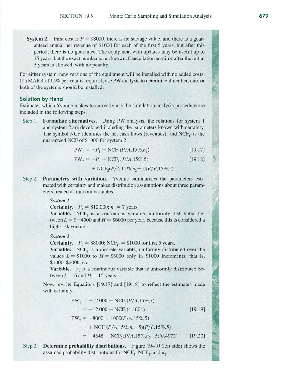
Step 3. Determine probability distributions. Figure 19-10 (left side) shows the
assumed probability distributions for NCF
j
,
NCF
z
, and n
2
•
679
680
CHAPTER
19
More on Variation and Decision Making Under Risk
/(NCF,)
1
10
Continuous
variable
- 4 - 2 0 2 4
NCF,,$IOOO
o
/(",)
...!..
9
6
4
NCF,,$IOOO
Continuous
variable
10
Figure
19-10
6
6
15
1.0
0.8
0.6
0.4
0.2
o
-4 -2
0 2 4 6
NCF,. $1000
F(NCF,)
1.00
0.83
0.67
0.50
0.33
II
0.17
o
F(",)
1.0
0.8
0.6
0.4
0.2
0
6
I
r
I
I
4
NCF,
. $1000
10
12
n2'
years
I
6
1415
Distributions used for random samples, Example
19
.7.
RN
RN
83-99
67
-8
2
50-66
33-49
17
- 3
2
00-1
6
RN
SECTION 19.5 Monte Carlo Sampling and Simulation Analysis
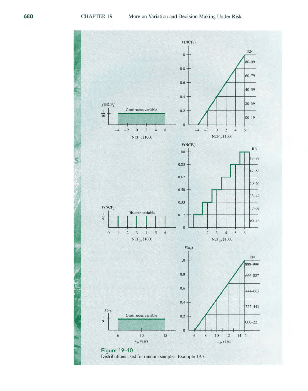
St
ep 4.
Random
sampling. Yvonne decides on a sample
of
size 30 and applies the
fir
st four
of
dle random sample steps
in
Section 19.3. Figure 19-10 (right
s
id
e) shows the cumulative distributions (step
1)
and assigns RNs to each
variable
(s
tep 2). The RNs for NCF
2
identify the x axis values so that all net
cash
Haws
will be
in
even $1000 amounts. For the continuous variable n
2
,
three
-di
git RN values are used
in
order to make the numbers come out
evenly, and they are shown in
ce
ll
s only
as
"indexers" for easy reference
when a RN is used to find a variable value. However, we round the number
to the next
hi
gh
er
value
of
n
2
because it
is
likely
lie
contract may be can-
celed on an anniversary date. Also, now the tabulated compound interest fac-
tors for
(n-z
-
5)
years can be used directly (see Table 19
-5).
Once the first RN is selected randomly from Table
19
-2,
the sequence
(step
3) used will be to proceed down the RN table column and then up the
column to the left. Table
19
-5
shows only the first five RN values selected
for each sample and the
cOl
Tesponding variable values taken from the cumu-
lat
iv
e
di
stributions
in
Figure
19
- 10 (step 4).
Step
5.
Measure
of
worth
calculation. With
th
e five sample values
in
Table 19- 5,
calc
ul
ate the PW values usi
ng
Equations [19.19] and [19.20].
1.
PW
1
= - 12,000 +
(-2200)(4.
1604)
2. PW
1
= -
12
,0
00 + 2000(4.1604)
3.
PW
1
= - 12,000 +
(-
1100)(4.1604)
4.
PW
1
= - 12,000 + (-900)(4.1604)
5.
PW
1
= - 12,000 + 3100(4.1604)
=
$-21,
153
=
$-3679
=
$-
16
,576
=
$-
15
,744
=
$+897
1.
PW
2
= - 4648 + 1000(P/A,
15
%,7)(0.4972) =
$-2579
2.
PW
2
= - 4648 +
1000
(P/A,
15%,5)(0.4972) =
$-298
1
3.
PW
2
= - 4648 + 5000(P/A,15%,8)(0.4972) =
$+6
507
4.
PW
2
= - 4648 +
30
00(PjA
,
15
%,
10)(0.4972) =
$+2838
5. PW
2
= - 4648 + 4000(P/A,15%,3)(0.4972) =
$-
107
TABLE
19-5
Random Numbers and Variable
Va
lues for NCF
,
.
NCF
2
•
and
/1
2'
Examp
le
.J
9.7
NCF
1
NCF
2
"2
RN*
Value
RNt
Value
RN:j:
Value
Rounde
d§
18
$-2200
10
$1000
586 11.3 12
59
+2000
10
1000 379 9.4
10
31
- 1100
77 5000 740
12
.7
13
29
-9
00
42 3000 967 14.4
15
71
+3
100
55
4000 144
7.
3
8
*Randomly start with row J, column 4
in
Table 1
9-2.
tStart with row 6, column
14.
tStart wi
th
row 4, column
6.
§T
he
11
2
va
lu
e is rounded up.
681
682 CHAPTER
19
More
on
Variation and Decision Making Under Risk
Now, 25 more RNs are selected for each variable from Table 19-2 and the
PW values are calculated.
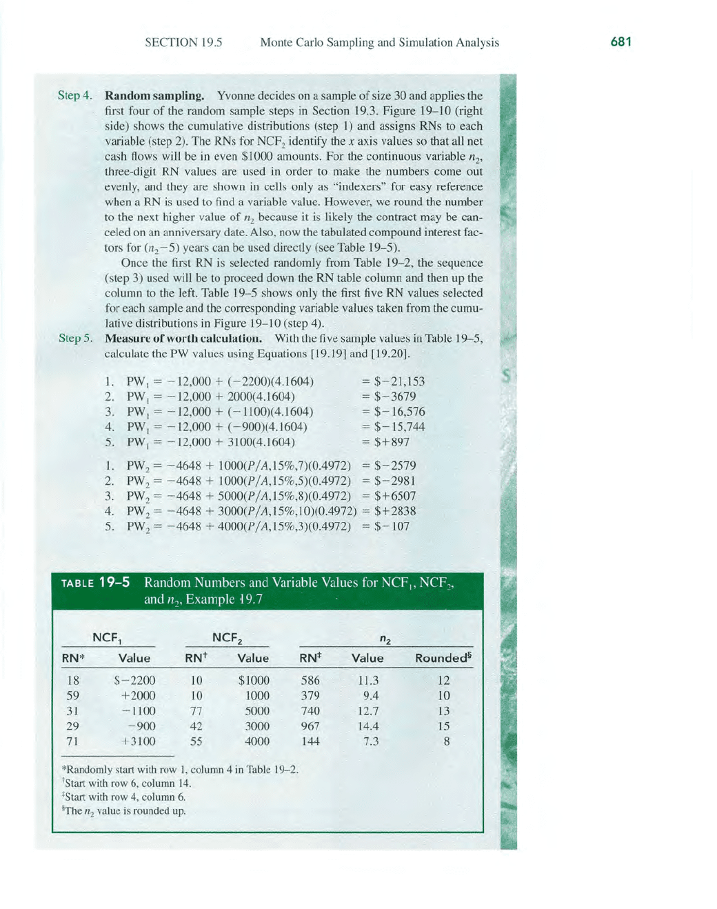
Step
6.
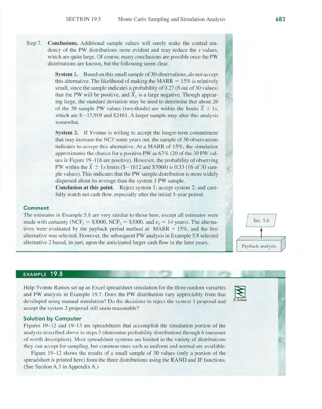
Measure of worth description. Figure 19-11a and b presents the
PW
I
and PW
2
probability distributions for the 30 samples with
14
and
15
cells,
respectively,
as
well
as
the range
of
individual PW values and the X and s
values.
Frequency
5
4
3
2
PW
1
•
Sample values range from $- 24,481 to
$+
12,962. The calcu-
lated measures
of
the 30 values are
XI
=
$-7729
s, = $10,190
PW
2
•
Sample values range from
$-3031
to
$+10
,324. The sample
measures are
-
r--
X
2
= $2724
S2 = $4336
XI
= $- 7729
111
= 30
sl
= $10,190
Range = $37,443
~PW
>
O
1
o
l-
t--
.
:
r--
h n
. . .
...
..
. . .
..
. ... ...
- 27 - 24 -
21
-
18
-15
-12
-9
-6
- 3 0 3
6
9
12
15
Frequency
6
5
4
3
2
1
o
- 4 - 3 - 2 - 1
Figure 19-11
PW
j
, $1000
Ca)
System 1
~PW
>
O
.
..
o
2
3
4 5
PW
2
,
$1000
(b) System 2
112
= 30
S2 = $4336
Range = $13,355
6 7 8 9
10
11
Probability distributions
of
simulated
PW
values for a sample
of
size 30, Example 19.7.
SECTION
19
.5
Monte Carlo Sampling and Simulation Analysis
Step 7. Conclusions. Additional sample values will surely make the central ten-
dency
of
the PW distributions more evident and may reduce the s values,
which are quite large.
Of
course, many conclusions are possible once the
PW
distributions are known, but the following seem clear.
Comment
System 1. Based on this small sample
of
30 observations, do nOl
accepl
this alternative. The likelihood
of
making the MARR =
15
%
is
relatively
small, since the sample indicates a probability
of
0.27 (8 out
of
30 values)
that the
PW will be positive, and
XI
is
a large negative. Though appear-
ing large, the standard deviation may be used
to
determine that about 20
of
the 30 sample PW values (two-thirds) are within the limits X
:±:
J s,
which are $- l7,9
19
and $2461. A larger sample may alter this analysis
somewhat.
System 2.
If
Yvonne
is
willing to accept the longer-term commitment
that may increase the NCF some years out, the sample
of
30 observations
indicates to
accept
this alternative. At a MARR
of
15%, the simulation
approximates the chance for a positive
PW
as
67% (20
of
the 30 PW val-
ues
in
Figure
19
-
11
b are positive). However, the probability
of
observing
PW
within the X
:±:
I s limits
($-1612
and $7060) is 0.53 (16
of30
sam-
ple values). This indicates that the
PW
sample distribution
is
more widely
dispersed about its average than the system 1
PW
sample.
Conclusion
at
this
point. Reject system
1;
accept system 2; and care-
fully watch net cash
flow,
especially after the initialS-year period.
The estimates
in
Example 5.8 are very similar to those here, except all estimates were
made with certainty (NCF
I
= $3000, NCF
2
= $3000, and
~
=
14
years). The alterna-
tives were evaluated by the payback period method at MARR
=
15
%, and the first
alternative was selected. However, the s
ub
sequent
PW
analysis
in
Example 5.8 selected
alternative 2 based,
in
part, upon the anticipated larger cash flow
in
the later years.
EXAMPLE
19.8
ii!l,
Help Yvonne Ramos set up
an
Excel spreadsheet simulation for the three random variables
and
PW
analysis
in
Example 19.7. Does the PW distribution vary appreciably from that
developed using manual simulation? Do the decisions to reject the system 1 proposal and
accept the system 2 proposal still seem reasonable?
Solution by
Computer
Figures
19
-
12
and
19
-13
are spreadsheets that accomplish the simulation portion
of
the
analysis described above
in
steps 3 (determine probability distribution) through 6 (measure
of
worth description). Most spreadsheet systems are limited
in
the variety
of
distributions
they can accept for
sa
mpling, but common ones such
as
uniform and normal are available.
Figure
19
-
12
shows the results
of
a small sample
of
30 values (only a portion
of
the
spreadsheet is printed here) from the three
di
stributions using the RAND and IF functions.
(See Section A.3 in Appendix A.)
683
Sec.5.6 I
Payback analysis
m
E·Solve
684
CHAPTER
19
More
on
Variation and Decision Making Under Risk
$6,000
$6,000
$2,000 507.36
11
36.8475
$3,000 681.54 13
83.461 $
000 369.092
10
77.8699
15
~
,9
~
go
91.3044 7
8.43079
$1,OgO
457.749
11
52.863,
$4000
914.543 15
+
~
57.4819
$4,000 698.762 13
$1
000 744.262 13
$5,000
190.§1~
\
8
$4,000 714.668: 13
RANDO* 1000 I
$4,000
648.227:
I
$6 199.949
1
=
IF(CI3
< =
16,
1000,lF(C
13
<
=32
,2000,TF(C
13
<
=49
,3000,
IF(C I 3< = 66,4000,IF(C
13
< = 82,5000,IF(C
13
< = 100,6000,6000» »)))
Figure 19- 12
Sample values generated using spreadsheet simulation, Example 19.8.
NCF
j
:
Continuous uniform from
$-4000
to $6000. The relation in column B trans-
lates RN
I values (column A) into NCFl amounts.
NCF
2
:
Discrete uniform in
$lOOO
increments from
$lOOO
to $6000. Column D cells
display NCF2
in
the $1000 increments using the logical IF function to translate from
the RN2 values.
n
2
:
Continuous uniform from 6
to
15
years. The results
in
column F are integer values
obtained using the INT function operating
on
the RN3 values.
Figure 19-13 presents the two alternatives' estimates
in
the top section. The PWI and PW2
computations for the 30 repetitions
of
NCFI,
NCF2, and n2 are the spreadsheet equiva-
lent
of
Equations [19.
19]
and [19.20]. The tabular approach used here tallies the number
of
PW values below zero ($0) and equal to or exceeding zero using the IF operator. For
example, cell
Cl7
contains a
1,
indicating
PWI
> 0 when
NCFl
= $3100 (in cell B7