Blank L., Tarquin A. Engineering Economy (McGraw-Hill Series in Industrial Engineering and Management)
Подождите немного. Документ загружается.

SECTION 19
.5
Monte Carlo Sampling a
nd
Simulation Analysis
X Microsoft Excel - Example
19
.8 I!lI'ij
~iew
Insert
FQrmat
lools
Qata
Yi,indow
f,-'§'
~~~
$8,000
n
yrs $1,000 5 yrs
MARR
1
5%
MARR
15
%
Results
of
Analysis
= SUMCHI
3:
H4
2)
10
19
#PW
< MARR 20
11
PWAverage ($7,10
5)
$1,649
=
AV
ERAGE(FI3:F42)
PVV
Std. Dev. $13,1
99
$3,871
= STDEV(F13:F42)
Present
Worth
Computations
PW1 ($23,649) 0 1
PW
2
$7,763
0
PW1
($
18,
24
1)
0 PW2
$202 1 0
PW1 ($24,897) 0 PW2
($885)
0
PW
1 ($12,832) 0 1 PW2
$2,045
0
PW1
$897
0
PW2 $5,352 1 0
PW1
($1,183)
0 PW2
($607)
0
PW1
($8 ,672)
0 PW2
($2,766)
0 1
($12,41
6)
$5,333
0
= - 8000-
PV
C
15
%,5, 1000)+
PVC
15
%,
5"
(PV(l5
%,'Random Numbers'!FI0- 5,'Random Numbers'IDIO)))
'-----i
= (
PV
($B$4,$B$3, - 'Random Numbers
"B
1O
))-$
B$2
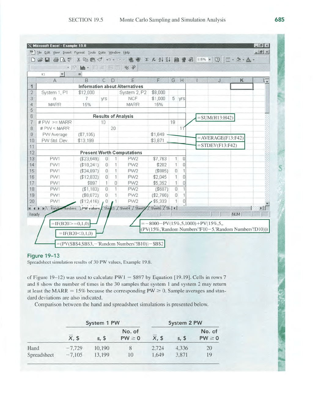
Figure
19-13
Spreadsheet simula
ti
on results of 30
PW
values. Example 19.8.
of
Figure
19
- 12) was used to c
al
culate
PW
1 = $897 by Equation [19.l91. Cells
in
rows 7
and 8 show the number
of
times
in
the
30
samples that system 1 and system 2 may return
at least the MARR
=
15
% because the corresponding
PW
:=::
O.
Sample averages and stan-
dard deviations are also indicated.
Comparison between the hand and spreadsheet simulations
is
presented below.
System
1
PW
System
2
PW
No.
of
No.
of
X,
$
5,
$
PW
:=::
O
X,$
5,
$
PW
:=::
O
Hand
- 7,729
10,190
8
2,724 4,336
20
Spreadsheet
- 7,105
13
,199
10
1,649 3,871
19
685
686
I
F(C
I
)
CHAPTER
19
More on Variation and Decision Making Under Risk
For the spreadsheet simulation,
10
(33%)
of
the
PWI
values exceed zero, while the man-
ual
simulation included 8 (27%) positive values. These comparative results will change
every time this spreadsheet
is
activated since the RAND function is set up (in this case)
to
produce a new RN each time. It
is
possible to define RAND to keep the same RN values.
See the Excel
User's Guide.
The conclusion to reject the system 1 proposal and accept system 2 is still appropriate
for the spreadsheet simulation as it was for the hand one, since there are comparable
chances that
PW
?
O.
ADDITIONAL EXAMPLES
PROBABILITY STATEMENTS, SECTION 19.2 Use the cumulative distribution for
th
e variable C
I
in
Figure
19-4
(Example 19.3, monthly cash flow for client I) to determine
the following probabilities:
(a) More than $14.
(b)
Between$12and$13.
(c) No more than
$11
or more than $14.
(d) Exactly $12.
Solution
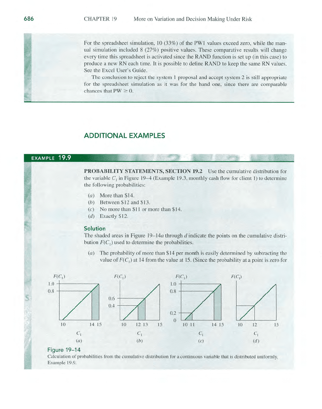
The shaded areas
in
Figure 19-14a through d indicate the points on the cumulative distri-
bution
F(C)
used to determine the probabilities.
(a) The probability
of
more than $14 per month
is
easily detennined by subtracting the
value
of
F(C
I
)
at
14
from the value at
15.
(Since the probability at a point is zero for
1.0
+
---
--
"7
0.8 +
----
-,(
F(C])
1.0+-----
,
0.8
+----
-,(
10
C
I
(a)
Figure
19-14
J4 15
0.6
+---
7f
0.4
+--
,(
10
12
13
C
l
(b)
15
0.2
o
10
11
14
IS
10
12
15
Calculation
of
probabilities from the cumulative distribution for a coutinuous variable that
is
distributed uniformly,
Example 19.9.
(b)
ADDITIONAL EXAMPLES
a continuous variable, the equals sign does not change the value
of
the resulting
probability.)
P(C
I
> 14) =
P(CI
::S
15)
-
P(CI
::S
14)
=
F(lS)
-
F(l4)
= 1.0 - 0.8
= 0.2
P(12
::S
C
I
::S
13) = P(CI::S 13) -
P(CI
::S
12) = 0.6 0.4
= 0.2
(c) P(CI
::S
11) +
P(CI
> 14) =
[F(ll)
-
F(lO)]
+
[F(IS)
-
F(14)]
(d)
= (0.2 - 0) + (1.0 - 0.8)
= 0.2 + 0.2
= 0.4
P(CI
= 12) =
F(l2)
-
F(l2)
= 0.0
There is no area under the cumulative distribution curve at a point for a continuous
variable, as mentioned earlier.
If
two very closely placed points are used, it is possi-
ble to obtain a probability, for example, between
12.0 and 12.1
or
between 12 and
13
, as
in
part (b).
EXAMPLE
19.10
I.',
THE NORMAL DISTRIBUTION, SECTION 19.4 Camilla is the regional safety
engineer for a chain
of
franchise-based gasoline and food stores. The home office has
had many complaints and several legal actions from employees and customers about
slips and falls due to liquids (water, oil, gas, soda, etc.) on concrete surfaces. Corporate
management has authorized each regional engineer to contract locall y to appl y to all ex-
terior concrete surfaces a newly marketed product that absorbs up to
100 times its own
weight in liquid and to charge a home office account for the installation.
The
authoriz-
ing letter to Camilla states that, based upon the.ir simulati.on and random samples that
assume a normal population, the cost
of
the locally arranged installation should be
about
$10,000 and almost always is within the range
of
$8000 to $12,000.
Camilla asks you, TJ, an engineering technology graduate, to write a
brief
but thor-
ough summary about the normal distribution, explain the
$8000 to $12,000 range state-
ment, and explain the phrase
"random samples that assume a normal population."
Solution
You
kept this book and a basic engineering statistics text when you graduated, and you
have developed the following response to Camilla, using them and the letter from the
home office.
Camilla,
Here is a brief summary
of
how the home office appears to be using the normal distribu-
tion. As a refresher,
I've
included a summary
of
what the normal distribution
is
all about.
687
688
CHAPTER
19
More
on
Variation and Decision Making Under Risk
Normal distribution, probabilities, and random samples
The normal distribution is also referred
to
as the bell-shaped curve, the Gaussian distri-
bution, or the error distribution. It is,
by
far, the most commonly used probability dis-
tribution in all applications.
It
places exactly one-half
of
the probability on either side
of
the mean or expected value. It is used for continuous variables over the entire range
of
numbers. The normal is found to accurately predict many types
of
outcomes, such
as
IQ values; manufacturing errors about a specified size, volume, weight, etc.; and the
distribution
of
sales revenues, costs, and many other business parameters around a
specified mean, which
is
why it may apply
in
this situation.
The normal distribution, identified
by
the symbol
N(J.L,(J2),
where
J.L
is the expected
value or mean and
(J2
is
the variance, or measure
of
spread, can be described as
follows:
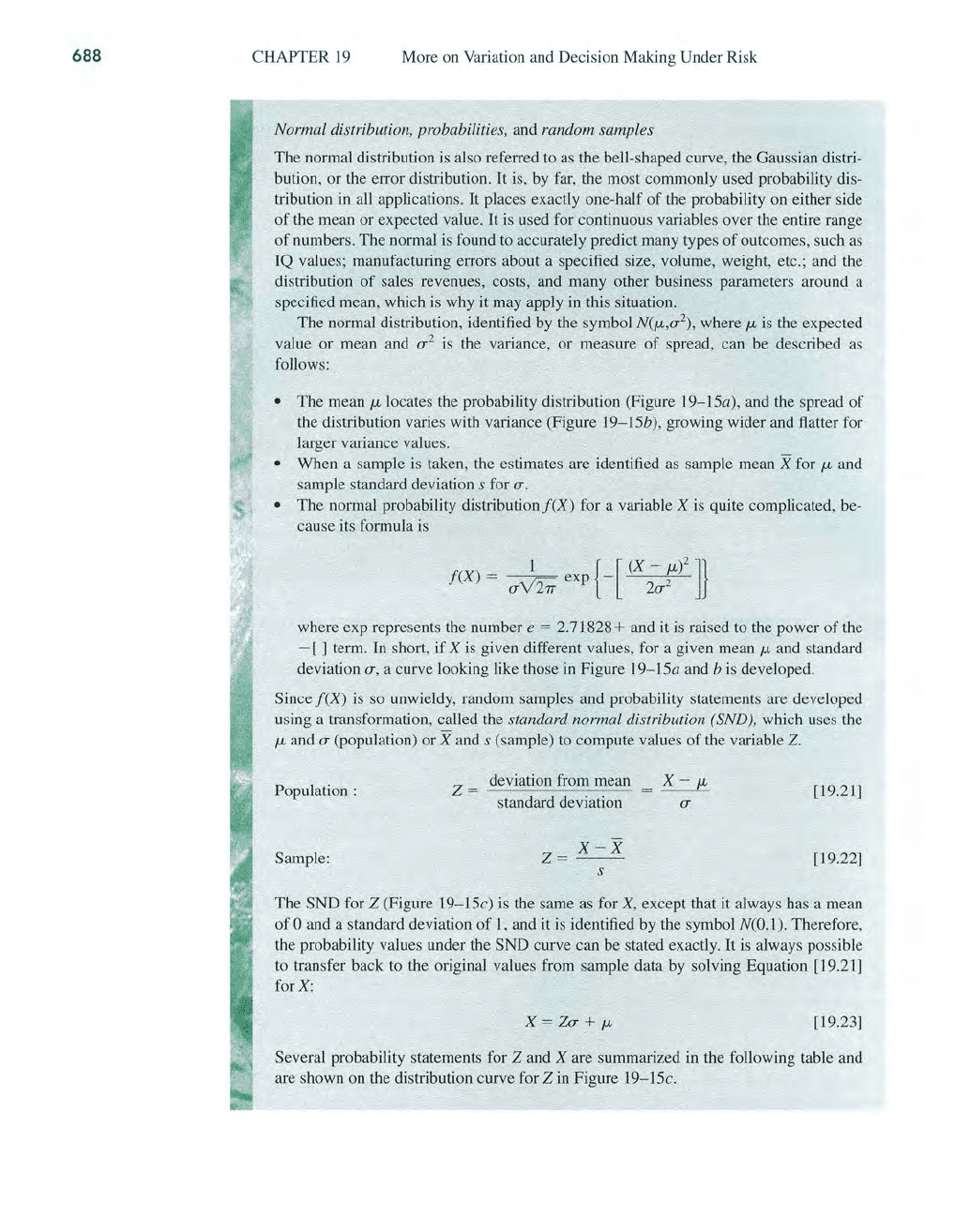
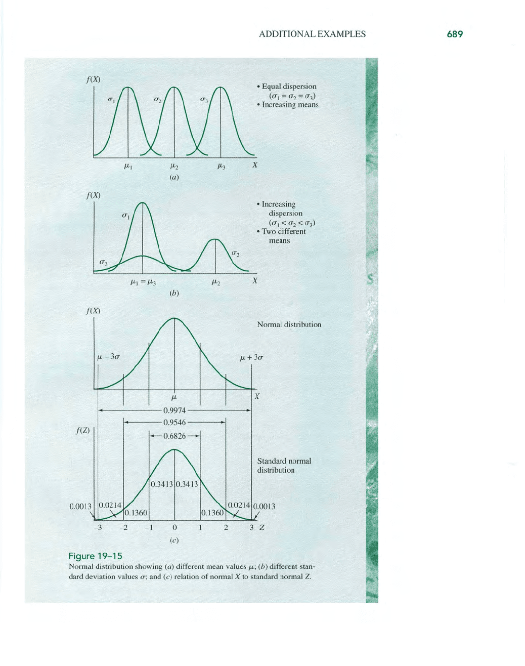
• The mean
J.L
locates the probability distribution (Figure 19-15a), and the spread
of
the distribution varies with variance (Figure 19-15b), growing wider and flatter for
larger variance values.
• When a sample
is
taken, the estimates are identified
as
sample mean X for
J.L
and
sample standard deviation
s for
(J.
• The normal probability distribution!(X) for a variable X is quite complicated, be-
cause its formula is
!(X)
=
(J~
exp
{_[
(X
~;)2]}
where exp represents the number e = 2.71828+ and it is raised
to
the power
of
the
- [ ] term.
In
short,
if
X
is
given different values, for a given mean
J.L
and standard
deviation
(J,
a curve looking like those in Figure 19-15a and b
is
developed.
Since
!(X)
is
so unwieldy, random samples and probability statements are developed
using a transformation, called the
standard normal distribution (SND), which uses the
J.L
and
(J
(population) or X and s (sample)
to
compute values of the variable
Z.
Population :
deviation from mean
__
X -
J.L
Z =
---------'-----'------------
standard deviation
(J
[19.21]
Sample:
X-X
Z=--
s
[19.22]
The
SND for Z (Figure 19-15c) is the same as for
X,
except that it always has a mean
of
° and a standard deviation
of
1, and it is identified
by
the symbol N(O,l). Therefore,
the probability values under the
SND curve can be stated exactly. It is always possible
to
transfer back
to
the original values from sample data
by
solving Equation
[19
.21]
for
X:
[19.23]
Several probability statements for
Z and X are summarized in the following table and
are shown on the distribution curve for
Z
in
Figure 19-15c.
f(X)
f(X)
(b)
f(X)
/J-
1------0
.
9974-------+1
feZ)
ADDITIONAL EXAMPLES
• Equal dispersion
(u
1
=u
2
= u
3
)
• Increasing means
• Increasing
dispersion
(u
1
<u2
< u3)
• Two different
means
x
Normal distribution
x
Standard normal
distribution
- 3
-2
- I
o
(c)
2 3 Z
Figure
19-15
Normal distribution showing (a) different mean values
/J-;
(b) different stan-
dard deviation values
u;
and (c) relation
of
normal X to standard normal
Z.
689
690
CHAPTER 19
More on Variation and Decision Mak
in
g Under
Ri
sk
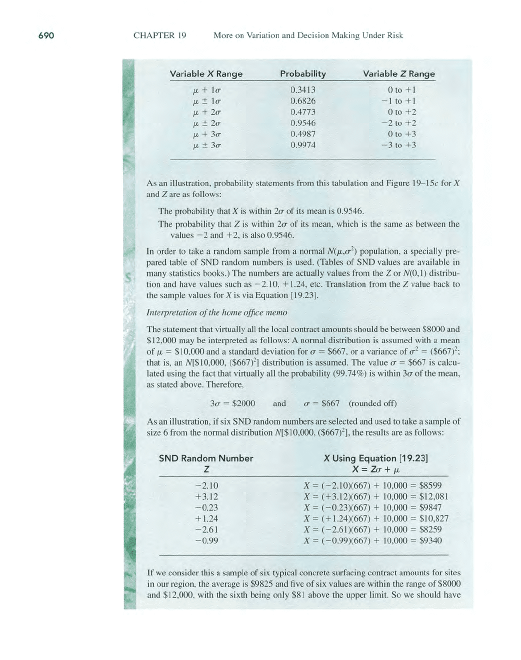
Variable X Range
Probability Variable Z Range
f-L
+
10-
0.3413 o to + 1
f-L
::'::
10-
0.6826
-I
to +1
f-L
+
20-
0.4773 o to
+2
f-L
::'::
2
0-
0
.9
546
-2
to
+2
f-L
+
30-
0.4987
o to
+3
f-L
::'::
30-
0.9974
-3
to
+3
As an illustration, probability statements from this tabulation and Figure
19
-
15
c
fo
r X
and
Z are
as
follow
s:
The probability that X
is
within
20-
of
its mean is 0.9546.
The probability
th
at Z
is
within
20-
of
its mean, which
is
the same as between the
values
- 2 and
+2,
is
also 0.9546.
In
order to take a random sample from a normal
N(f-L,0-
2)
population, a specially pre-
pared table
of
SND random numbers is used. (Tables
of
SND values are available
in
many sta
ti
s
ti
cs books.) The numbers are actually values from
th
e Z or N(O,I) distribu-
tion and have values such
as
-2.
10
, + 1.24, etc. Translation from the Z value back to
th
e sample values for X
is
via Equation
[19
.23
].
Interpretation
of
the home office memo
The statement that virtually all the local contract amounts should be between
$8000 and
$
12
,000 may be interpreted
as
follows: A normal distribution
is
assumed with a mean
of
f-L
= $
10
,000 and a standard deviation for
0-
= $667, or a variance
of
0-
2
= ($6
67
?;
th
at is,
an
N[$ I 0,000,
($
667
)2
]
di
stribution is assumed. The
va
lu
e
0-
= $667 is calcu-
lat
ed
us
in
g the fact that virtually a
ll
the probability (99.74%) is within
30-
of
the mean,
as
stated above. Therefore,
30-
= $2000 and
0-
= $667 (rounded off)
As
an
illustration, if six SND random numbers are selected and used to take a sample
of
size 6 from the normal distribution N[$IO,
OOO
, ($667)2], the results are
as
follows:
SND Random Number
Z
- 2.10
+ 3.12
- 0
.23
+
1.
24
- 2.61
-0.99
X Using Equation [19.23)
X=Zo-+f-L
X =
(-
2.10)(667) + 10,000 = $8599
X = (+3.12)(667) +
10
,0
00 = $12,081
X = (-0.23)(667) + 10,000 = $9847
X =
(+
1.24)(667) +
10
,000 = $10,827
X =
(-2.6
1)(667) + 10,000 = $8259
X =
(-
0.99)(667) +
10
,000 = $9340
If
we consider this a sample
of
six typical concrete surfacing contract amounts for sites
in
our region, the average is $9825 and five
of
six values are within the range of $8000
and $
12
,000, with
th
e six
th
being only
$81
above the upper limit. So we should have
PROBLEMS
no
real problems, but
it
is
important that we keep a close watch on the contract
amounts, because the assumption
of
the normal distribution wi
th
a mean
of
about
$10,000 and virtually all contract amounts within :':$2000
of
it
may not prove to be
correct for ollr regi
on
.
If
YOll
have any questions abollt this summary, please contact me.
T]
;:,
or,:
:: '
CHAPTER
SUMMARY
To
perform decision making under risk implies that some parameters
of
an engi-
neering alternative are treated as random variables. Assumptions about the shape
of
the variable's probability distribution are used to explain how the estimates
of
parameter values may vary. Additionally, measures such as the expected value
and standard deviation describe the characteristic shape
of
the distribution.
In
this
chapter, we learned several
of
the simple, but useful, discrete and continuous pop-
ulation distributions used in engineering
economy-uniform
and
triangular-as
well as specifying our own distribution or assuming the normal distribution.
Since the population's probability distribution for a parameter is not fully
known, a random sample
of
size n
is
usually taken, and its sample average and
standard deviation are determined. The results are used to make probability
statements about the parameter, which help make the final decision with risk
considered.
The Monte Carlo sampling method
is
combined with engineering economy
relations for a measure
of
worth such as
PW
to implement a simulation approach
to risk analysis. The
re.' 'Its
of
such an analysis can then be compared with deci-
sions when parameter
. ,' imates are made with certainty.
PROBLEMS
691
Certainty, Risk, and Uncertainty
19.1
For each situation below, determine
(l)
if
the variable(s) is(are) discrete
or
continu-
ous and (2)
if
the information involves
certainty, risk, and/or uncertainty. Where
risk is involved, graph the information in
the general form
of
Figure 19-1,
will go up slowly or rapidly during
the next 6 months.
(a) A friend
in
real estate tells you the
price per square foot for new houses
(b) Your manager informs the staff there
is an equal chance that sales will be
between 50 and
55
units next month.
(c) Jane got paid yesterday, and $400
was taken out in income taxes. The
amount withheld next month will be
larger because
of
a pay raise between
3%and5%.
692
CHAPTER
19
More
on Variation and Decision
Making
Under
Risk
(d)
There is a 20% chance
of
rain and a
30
% chance
of
snow today.
19.2 An engineer learned that production out-
put
is
between 1000 and 2000 units per
week
90%
of
the time, and it may fall
below
1000
or
go
above 2000. He wants
to use E(output)
in
the decision making
process. Identify at least two additional
pieces
of
information that must be ob-
tained
or
assumed to finalize the output
information for this use.
Probability
and
Distributions
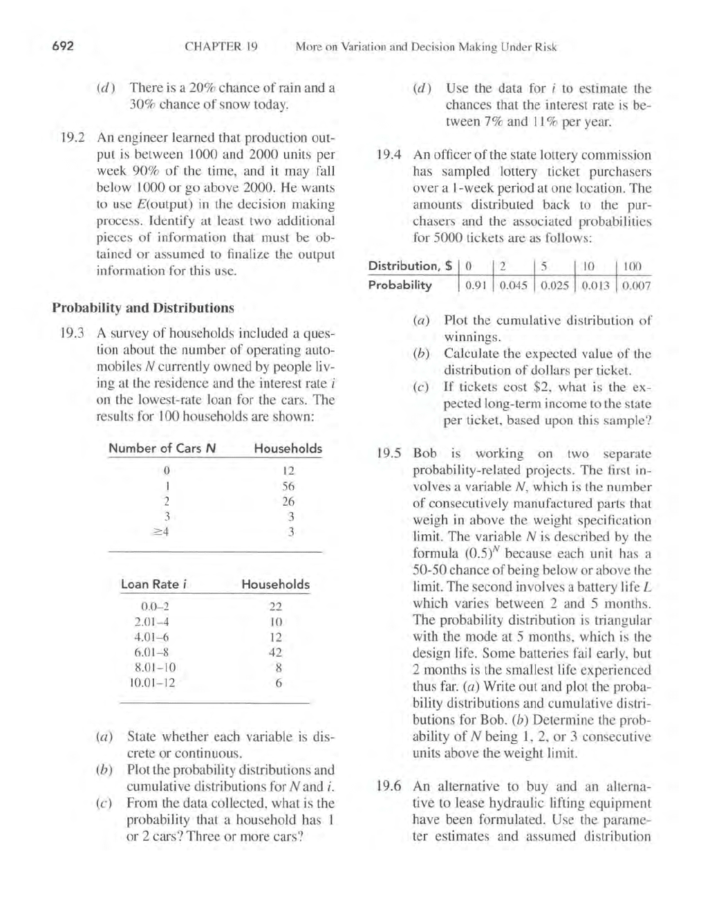
19.3 A survey
of
households included a ques-
tion about the numb
er
of
operating auto-
mobiles
N currently owned by people liv-
ing at the residence and the interest rate
i
on the lowest-rate loan for the cars. The
results for
100 households are shown:
Number
of
Cars N
o
I
2
3
2':
4
Loan
Rate;
0.0-2
2.01
- 4
4.01- 6
6.01- 8
8.01
-
10
10.01
-
12
Households
12
56
26
3
3
Households
22
10
12
42
8
6
(a) State whether each variable is dis-
crete
or
continuous.
(b)
Plot the probability distributions and
cumulative distributions for
Nand
i.
(c) From the data co
ll
ected, what is the
probability that a household has 1
or
2 cars? Three
or
more cars?
(d)
Use the data for i to estimate the
chances that the interest rate
is
be-
tween
7%
and
11
% per year.
19.4 An officer
of
the state lottery commission
has sampled lottery ticket purchasers
over a
I-week
period at one location.
The
amounts distributed back to the pur-
chasers and the associated probabilities
for
5000 tickets are as follows:
Distribution, $
100
Probability
0.007
(a) Plot the cumulative distribution
of
winnings.
(b) Calculate the expected value
of
the
distribution
of
dollars per ticket.
(c)
If
tickets cost $2, what is the ex-
pected long-term income to the state
per ticket, based upon this sample?
19.5 Bob
is
working on two separate
probability-related projects.
The
first in-
volves a variable
N,
which
is
the number
of
consecutively manufactured parts that
weigh
in
above the weight specification
limit.
The
variable N
is
described by the
formula
(0.5)N because each unit has a
50-50 chance
of
being below
or
above the
limit.
The
second involves a battery life L
which varies between 2 and 5 months.
The
probability distribution
is
triangular
with the mode at 5 months, which is the
design life.
Some
batteries fail early, but
2 months
is
the smallest life experienced
thus far.
(a) Write out and plot the proba-
bility distributions and cumulative distri-
butions for Bob.
(b) Determine the prob-
ability
of
N being
1,2
,
or
3 consecutive
units above the weight limit.
19.6 An alternative to buy and an alterna-
tive to lease hydraulic lifting equipment
have been formulated.
Use the parame-
ter estimates and assumed distribution
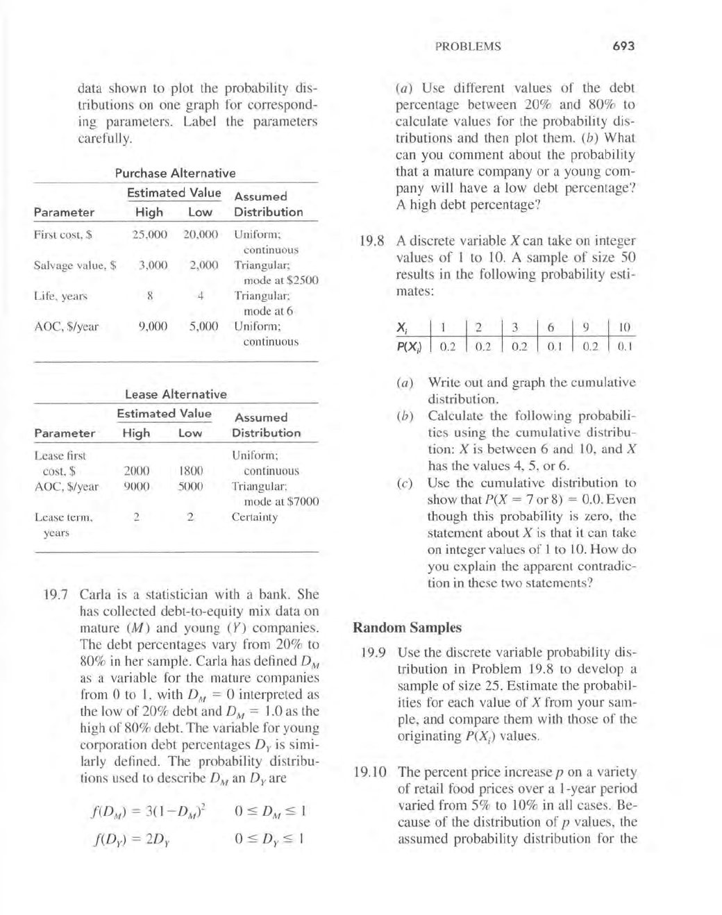
data shown to plot the probability dis-
tributions on
one
grap
h for correspond-
in
g parameters. Label the parameters
carefully.
Purchase
Alternative
Estimated
Value
Assumed
Parameter
High
Low
Distribution
First cost, $ 25,000 20,000
Uniform;
continuous
Salvage value, $
3,000 2,000
Triangular;
mode at
$2500
Life, years
8
4 Triangular;
mode at 6
AOC, $/year
9,000 5,000 Uniform;
continuous
Lease
Alternative
Estimated
Value
Assumed
Parameter
High
Low
Distribution
Lease first
Uniform;
cost, $
2000 \800 cont
inu
ous
AOC, $/year 9000 5000
Triangular;
mode at
$7000
Lease term, 2 2
Certainty
years
19
.7
Carla
is
a statistician with a bank.
She
has collected debt-to-equity mix data on
mature
(M)
and young (Y) companies.
The
debt percentages vary from
20%
to
80%
in
her sample. Carla has defined
DM
as a variable for the mature
companies
from 0 to I, with
DM
= 0 interpreted as
the low
of
20%
debt
and
DM
=
J.O
as the
high
of
80% debt.
The
variable for
young
corporation
debt
percentages
Dy
is simi-
larly defined.
The
probability distribu-
tions used to describe
DM
an
Dy
are
f(D
M
)
=
3(I-D
M
)2
f(Dy) = 2Dy
0::::;
D
M
::::;
0::::;
Dy::::;
I
19.8
PROBLEMS 693
(a)
Use
different values
of
the
debt
percentage
between
20
% and 80% to
calculate values for the probability dis-
tributions and
then
plot
them.
(b)
What
can you
comment
about
the probability
that a mature
company
or
a
young
com-
pany will have a
low
debt
percentage?
A high
debt
percentage
?
A discrete variable X
can
take on integer
values
of
I to
10.
A
sample
of
size
50
results in the following probability esti-
mates:
0.2 0.2
O.
\ 0.2 0.\
(a) Write
out
and graph the cumulative
distribution.
(b) Calculate the following probabili-
ties using the
cumulative
distribu-
tion: X is between 6 and 10, and X
has the values 4, 5,
or
6.
(c)
Use
the cumulative distribution to
show that
P(X
= 7
or
8) = 0.0.
Even
though this probability
is
zero, the
statement about X is that it can take
on integer values
of
I to
10.
How
do
you explain the apparent contradic-
tion in these two statements?
Random
Samples
19.9 Use the discrete variable probability dis-
tribution
in
Problem 19.8 to develop a
sample
of
size 25. Estimate the probabil-
ities for each value
of
X from
your
sam-
ple, and
compare
them
with those
of
the
originating
P(X)
va
lue
s.
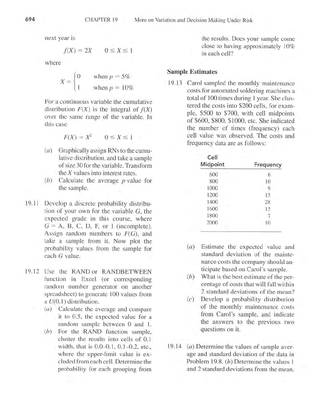
19.10
The
percent price increase p on a variety
of
retail food prices
over
a
I-year
period
varied from
5%
to
10
% in all cases. Be-
cause
of
the distribution
of
p values, the
assumed probability distribution for the
694
CHAPTER
19
More
on Variation and Decision
Making
Under Risk
next year is
f(X)
=
2X
where
x =
(~
when p = 5%
whenp
= 10%
For a continuous variable the cumulative
distribution
F(X)
is
the integral
of
f(X)
over the same range
of
the variable. In
this case
F(X)
=
X2
(a) Graphically assign RNs to the cumu-
lative distribution, and take a sample
of
size 30 for the variable. Transform
the X values into interest rates.
(b)
Calculate the average p value for
the sample.
19
.
11
Develop a discrete probability distribu-
tion
of
your own for the variable G, the
expected grade in this course, where
G
=
A,
B, C, D,
F,
or I (incomplete).
Assign random numbers to
F(G), and
take a sample from
it.
Now plot the
probability values from the sample for
each G value.
19.
12
Use the
RANDor
RANDBETWEEN
function
in
Excel (or corresponding
random number generator on another
spreadsheet) to generate
100 values from
a U(O,1) distribution.
(a)
Calculate the average and compare
it to
0.5, the expected value for a
random sample between
0 and
1.
(b) For the RAND function sample,
cluster the results into cells
of
0.1
width, that
is
0.0-0.1, 0.1-0.2, etc.,
where the upper-limit value
is
ex-
cI
uded from each cell. Determine the
probability for each grouping from
the results. Does your sample come
close to having approximately
10%
in each cell?
Sample Estimates
19.
13
Carol sampled the monthly maintenance
costs for automated soldering machines a
total
of
100 times during 1 year. She clus-
tered the costs into
$200 cells, for exam-
ple,
$500 to $700, with cell midpoints
of
$600, $800, $1000, etc. She indicated
the number
of
times (frequency) each
cell value was observed.
The
costs and
frequency data are as follows:
Cell
Midpoint
Frequency
600
6
800
10
1000
9
1200
15
1400
28
1600
15
1800
7
2000
10
(a)
Estimate the expected value and
standard deviation
of
the mainte-
nance costs the company should an-
ticipate based on Carol's sample.
(b)
What is the best estimate
of
the
per
-
centage
of
costs that will fall within
2 standard deviations
of
the mean?
(c) Develop a probability distribution
of
the monthly maintenance costs
from Carol's sample, and indicate
the answers to the previous two
questions on
it.
19.1
4
(a)
Determine the values
of
sample aver-
age and standard deviation
of
the data
in
Problem 19.8. (b) Determine the values 1
and 2 standard deviations from the mean.