Blank B.E., Krantz S.G. Calculus: Single Variable

Подождите немного. Документ загружается.

Computer/Calculator Exercises

87. Using Theorem 3, we obtain

lim

x-2

2 2:9x 1 2

5 40:

As x-2

about how close to 2 must x be to ensure that

2 2:9x 1 2

2 40



, 0:1?

Illustrate this by a graph of f ðxÞ5 x

=ðx

2 2:9x 1 2Þ in an

appropriate viewing rectangle.

88. It can be shown that

lim

x-π

ﬃﬃﬃﬃﬃﬃﬃﬃﬃﬃﬃ

x 2 π

ﬃﬃﬃﬃﬃﬃﬃﬃﬃﬃﬃﬃﬃﬃﬃ

sinð2xÞ

ﬃﬃﬃ

Find an interval I with center π such that

ﬃﬃﬃﬃﬃﬃﬃﬃﬃﬃﬃ

x 2 π

ﬃﬃﬃﬃﬃﬃﬃﬃﬃﬃﬃﬃﬃﬃﬃ

sinð2xÞ

ﬃﬃﬃ



, 0:01

for x in I. Illustrate this by a graph of f ðxÞ5

ﬃﬃﬃﬃﬃﬃﬃﬃﬃﬃﬃﬃﬃﬃ

x 2 π=

p ﬃﬃﬃﬃﬃﬃﬃﬃﬃﬃﬃﬃﬃﬃﬃ

sinð2xÞ

in an appropriate viewing rectangle.

89. Calculate ‘ 5 lim

x-2

ðx

2 3x

1 2x 1 1Þ. Find an interval

I with center 2 such that

jðx

2 3x

1 2x 1 1Þ2 ‘j, 0: 1

for x in I. Illustrate this by a graph of f ðxÞ5 x

1 2x 1 1 in an appropriate viewing rectangle.

90. Verify that lim

x-1



=ðx 1 1Þ



5 1. For ε 5 1=100, use a

computer algebra system to determine exactly what δ (in

the deﬁnition of limit) should be.

91. Graph gðxÞ5 sinðx



Þ=x for 245 # x # 45 where x



means “x degrees.” Use your graph to determine the

value of lim

x-0

gðxÞ.

92. Graph gðxÞ5



1 2 cosðx



for 245 # x # 45, where



means “x degrees.” Use your graph to determine the

value of lim

x-0

g ðxÞ:

c In each of Exercises 93296, plot the given functions g, f,

and h in

a common viewing rectangle that illustrates f being

pinched at the point c. Determine lim

x-c

f ðxÞ: b

93. gðxÞ5 2; f ðxÞ5 2 1 ðx21Þ

cos



x=ðx 2 1Þ



;

hðxÞ5 2 1 jx 2 1j=4 c 5 1

94.



xÞ5 ðx 2 2Þ

; f



xÞ5 ðx 2 2Þ



2 1 sin



tanðπ=xÞ







ðx 2 2Þ

; hðx



5 3ðx 2 2Þ

c 5 2

95. gðxÞ522jxj; f ðxÞ5 cosðx 2 1=xÞ2 cosðx 1 1=xÞ;

hðxÞ5 2jxj c 5 0

96. gðxÞ5 2 2 4jxj; f ðxÞ5 ð2 1 x

Þ=ð1 1 x

Þ1 sinðx 1 1=xÞ1

sinðx 2 1=xÞ; hðxÞ5 2ð1 1 jxjÞ c 5 0

2.3 Continuity

When we drive along a high-speed road, we frequently cannot see very far ahead.

We learn to drive as though the portion of the road immediately beyond our vision

is the obvious extension of the portion of the road that we can see. What we are

doing is computing the limit of what we see. Usually, the actual state of the road

coincides with what we have anticipated it will be (i.e., the road is continuous). If

the road has been damaged, or if a bridge is out, then the actual state of the road

does not coincide with what we have anticipated (the road is discontinuous). In this

section, we develop mathematical analogues of these ideas.

The Deﬁnition of

Continuity at a Point

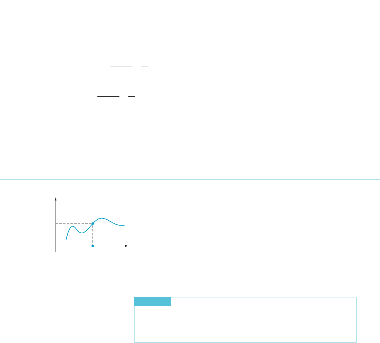
Here is a precise deﬁnition of continuity of a function at a point.

DEFINITION

Suppose a function f is deﬁned on an open interval that contains

the point c. We say that f is continuous at c, provided that

lim

x-c

f ðxÞ5 f ðcÞ:

See Figure 1.

f (c)

m Figure 1 f (x) has the limit

f (c)asx tends to c.

2.3 Continuity 105

INSIGHT

When we say that f is continuous at c, we are asserting three things:

1. f is deﬁned at c;

2. there is a certain value

lim

x-c

f ðxÞ that we expect f to take at c (i.e., lim

x-c

f ðxÞ

exists); and

3. the expected value lim

x-c

f ðxÞ agrees with the value f (c) which value f actually

takes at c (lim

x-c

f ðxÞ5 f ðcÞ).

We consider continuity of a function only at points of its domain. For instance,

we would not say that the function f ðxÞ5 sinðxÞ=x is continuous at 0 because 0 is

not in the domain of f. If a point c is in the domain of f,andf is not continuous at c,

then we say that f is discontinuous at c. Such a point is called a point of discontinuity

of f.Ifc is a point of discontinuity of f, then either f (x) does not have a limit as x

approaches c, or the limit exists but is not equal to f (c).

When a function f is continuous at every point of its domain, then we say that f is

a continuous function. The theorems about limits that were developed in Section 2.2

show that polynomials, rational functions, n

roots, and trigonometric functions are

continuous functions.

An Equivalent

Formulation of

Continuity

The continuity of f at c can be expressed in another form. Let Δx denote an

increment in x. Write x 5 c 1 Δx; and observe that x-c is equivalent to Δx-0.

With this notation, the continuity of f at c is equivalent to

lim

Δx-0

f ðc 1 Δ x Þ5 f ðcÞ:

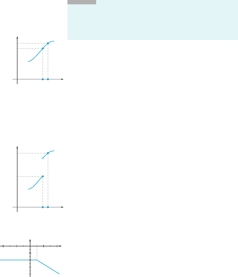
Imagine an experiment to determine the mass y 5 f(x) of a compound that is

produced by a chemical reaction with a substance that has mass x. Suppose the

value of x in the experiment is taken to be c. Inevitably, there will be a small

measurement error Δx. With care, the actual value of x, c 1 Δx, will be close to the

desired value c, but it will usually not be exactly c . Although the result of

the experiment is intended to be f (c), it is really f ðc 1 ΔxÞ. However, the result

of the experiment is not necessarily unreliable. If c is a value at which f is con-

tinuous, then the difference between f ðc 1 ΔxÞ an d f (c) can be made small by

controlling the size of the measurement error Δx. In other words, sufﬁciently small

errors in the independent variable x result in correspondingly small errors in the

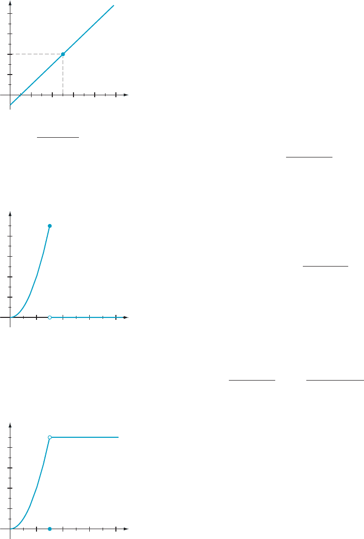
dependent variable y (see Figure 2). By contrast, if c is a point at which f is

discontinuous, then a very small nonzero value of Δx can result in a substantial

error, f ðc 1 ΔxÞ2 f ðcÞ,

in the outcome of the experiment (see Figure 3).

⁄ EX

AMPLE 1 Let

FðxÞ5

24i

fx , 1

2x 2 3ifx $ 1



Verify that F is co ntinuous at every c in R.

Solution If c , 1,

then

lim

x-c

FðxÞ5 lim

x-c

ð24Þ524 5 FðcÞ:

f (c)

(c  x)

c  x

m Figure 2 A small input error

near a point of continuity results

in a small output error.

f (c)

f (c  x)

c  x

m Figure 3 A small input error

near a point of discontinuity can

result in a large output error.

2442

2

8

6

m Figure 4

106 Chapter

2 Limits

If c . 1, then

lim

x-c

FðxÞ5 lim

x-c

ð2x 2 3Þ52c 2 3 5 FðcÞ:

If c 5 1, then we see, by checking both on the left and on the right, that

lim

x-1

FðxÞ5 lim

x-1

ð24Þ524 5 Fð1Þ and lim

x-1

FðxÞ5 lim

x-1

ð2x 2 3Þ524 5 Fð1Þ:

Therefore F is continuous at every c in R (see Figure 4).

⁄ EX

AMPLE 2 Let

FðxÞ5

2 6x 1 5

x 2 5

if x 6¼ 5

4ifx 5 5

Is F a continuous function?

Solution We

must investigate F at each point c of its domain R. First suppose that

c 6¼ 5. Because the denominator of F(x) is never 0 when x is near such a value of c,

we may apply Theorem 2c from Section 2.2:

lim

x-c

FðxÞ5

2 6c 1 5

c 2 5

5 FðcÞ:

Next we consider c 5 5. Remember that, when we compute lim

x-5

FðxÞ; we use

values of x near 5 but not equal to 5. Consequently, the quantity x 2 5 is nonzero.

Observe that this expression appears not only in the denominator of F(x), but also

in the numerator x

2 6x 1 5, which factors as ðx 2 5Þðx 2 1Þ. Of course, any

nonzero expression that appears in both the numerator and denominator of a

fraction may be cancelled. Therefore

lim

x-5

FðxÞ5 lim

x-5

2 6x 1 5

x 2 5

5 lim

x-5

ðx 2 5Þðx 2 1Þ

x 2 5

5 lim

x-5

ðx 2 1Þ5 4 5 Fð5Þ;

which shows that F is continuous at c 5 5. In summary, we have demonstrated that F is

continuous at every point of its domain. By deﬁnition, it follows that F is a continuous

function. Figure 5 shows the graph of F in the viewing window [0, 10] 3 [21, 9].

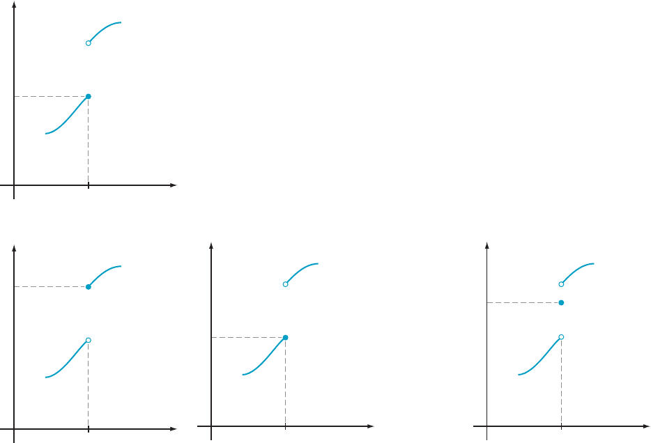
⁄ EX

AMPLE 3 Let

GðxÞ5

if x , 3

9ifx 5 3

0ifx . 3

and HðxÞ5

if x , 3

0ifx 5 3

9ifx . 3

See Figures 6 and 7. Discuss the continuity of G and H at c 5 3.

Solution Obser

ve that lim

x-3

GðxÞ does not exist because lim

x-3

GðxÞ5 0and

lim

x-3

GðxÞ5 9: So it is certainly not the case that lim

x-3

GðxÞ5 G ð3Þ: Thus G is

discontinuous at c 5 3. Although lim

x-3

HðxÞ exists, lim

x-3

HðxÞ5 9 6¼ Hð3Þ.

Therefore H is also discontinuous at c 5 3.

104682

y  F(x)

m Figure 5

FðxÞ5

2 6x 1 5

x 2 5

if x 6¼ 5

4ifx 5 5

84362

y  G(x)

m Figure 6

GðxÞ5

if x , 3

9ifx 5 3

0ifx . 3

84362

y  H(x)

m Figure 7

HðxÞ5

if x , 3

0ifx 5 3

9ifx . 3

2.3 Continuity 107

⁄ EXAMPLE 4 Show that the function

FðxÞ5

sinðxÞ

if x 6¼ 0

1ifx 5 0

is continuous at c 5 0.

Solution Theor

em 8 from Section 2.2 tells us that lim

x-0

FðxÞ5 1 5 Fð0Þ. Thus F

is continuous at 0 (see Figure 8).

Continuous Extensions Consider a continuous function f that is deﬁned on an interval (a, c) to the left of c

and on an interval (c, b) to the right of c. Can we assign a value to f at c to create a

continuous function on ða; bÞ? More precisely, is there a continuous function F that

is deﬁned on the entire interval ða; bÞ such that FðxÞ5 f ðxÞ for x 6¼ c? The answer

is that F exists precisely when lim

x-c

f ðxÞ exists. If we let ‘ 5 lim

x-c

f ðxÞ, then the

function F deﬁned by

FðxÞ5

f ðxÞ if x 6¼ c

‘ if x 5 c



is continuous. We refer to F as the continuous extension of f. This situation is illustrated

in Figure 9. Because the domain of F is larger than the domain of f, we see that F is not

the same function as f. Refer back to Example 2, and you will see that the function F of

that example is a continuo us extension of x/ðx

2 6x 1 5Þ= ðx 2 5Þ. Similarly, the

function F of Example 4 is a continuous extension of x/sinðxÞ=x.

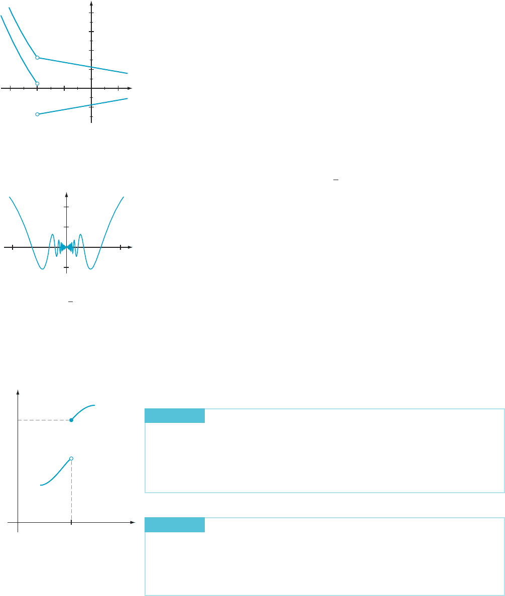
⁄ EX

AMPLE 5 Let

f ðxÞ5

2 14 if x ,24

x 1 7ifx .24

and gðxÞ5

2 3ifx ,24

9 2 x if x .24



Is it possible to deﬁne a continuous extension of f ?Ofg?

Solution Because,

the left limit, lim

x-ð24Þ

f ðxÞ5 ð24Þ

2 14 5 2, and the right

limit, lim

x-ð24Þ

f ðxÞ5 ð24Þ1 7 5 3, are unequal, we see that lim

x-24

f ðxÞ does not

exist. Therefore no continuous extension exists. On the other hand, as x

approaches 24 from the left, the value gðxÞ5 x

2 3 approaches 13. In addition,

0.98

0.96

0.50.5

m Figure 8

Fð xÞ5

sinðxÞ

if x 6¼ 0

1ifx 5 0

m Figure 9a

m Figure 9b The continuous extension of f

108 Chapter 2 Limits

as x approaches 24 from the right, the value gð x Þ5 9 2 x also approaches 13. Thus

lim

x-24

gðxÞ5 13, and the function

GðxÞ5

gðxÞ if x 6¼24

if x 524



is a continuous extension of g. The graphs of f and g (see Figure 10) clearly

illustrate the different behaviors of the functions at x 524.

We sometimes say that a function is continuous if its graph has no “jumps” or if

the graph can be drawn without lifting the pencil from the paper. These intuitive

concepts are helpful in treating some of the preceding examples. However, the

continuous function

FðxÞ5

x  sin





if x 6¼ 0

0ifx 5 0

that we considered in Example 6 from Section 2.2 is much more difﬁcult to

understand in this informal manner. The graph oscillates rapidly near the origin, as

shown in Figure 11, and the truth is that we cannot really draw the graph with or

without lifting the pencil from the paper. It is precisely because of funct ions like

these that we have gone to the trouble of learning careful deﬁnitions of “limit” and

“continuous.” These careful deﬁnitions enable us to say exactly at which points a

function is continuous and at which points it is not.

One-Sided Continuity In calculus, we frequently study functions that are deﬁned on intervals that have an

endpoint. In such cases, we can approach the endpoint only from one side. There

are other situations in which we can approach a point in the domain from each side,

but the behavior of the function is quite different on the two sides. We require a

concept of continuity that is appropriate for such cases.

DEFINITION

Suppose f is a function with a domain that con tains ½c; bÞ.If

lim

x-c

f ðxÞ5 f ðcÞ;

then we say that f is continuous from the right at c,orf is right-continuous at c.

Figure 12 exhibits a function that is right-continuous at c.

DEFINITION

Suppose f is a function with a domain that con tains ða; c.If

lim

x-c

f ðxÞ5 f ðcÞ;

then we say that f is continuous from the left at c,orf is left-continuous at c.

Figure 13 shows a function that is left-continuous a t c.

8

26 4 2

m Figure 10

f ðxÞ5

2 14 if x ,24

x 1 7ifx .24



gðxÞ5

2 3ifx ,24

9 2 x if x .24



f (c)

m Figure 12 f is right-

continuous at c.

0.4

0.2

0.2

0.50.5

m Figure 11

FðxÞ5

x  sin





if x 6¼ 0

0ifx 5 0

2.3 Continuity 109

Just as in the deﬁnition of continuity, the notions of left and right continuity at c

entail three requirements:

1. The point c is in the domain of f.

2. The one-sided limit at c exists.

3. The one-sided limit must equal f ðcÞ.

Also notice that “f is continuous at c” is equivalent to “f is left continuous at c and

right-continuous at c.” If lim

x-c

f ðxÞ and lim

x-c

f ðxÞ both exist but are different

numbers, then f is said to have a jump discontinuity at c (see Figure 14).

⁄ EX

AMPLE 6 Is the function

gðxÞ5

2x if x , 4

if x $ 4



continuous from the left at 4? Is it continuous from the right at 4?

Solution The

function g satisﬁes

lim

x-4

gðxÞ5 lim

x-4

2x 5 8 6¼ 16 5 gð4Þ:

Thus g is not continuous from the left at 4. However,

lim

x-4

gðxÞ5 lim

x-4

5 16 5 gð4Þ:

Therefore g is continuous from the right at 4.

Some Theorems about

Continuity—Arithmetic

Operations and

Composition

Our work with the concept of continuity would be tedious if we had to check, from

the deﬁnition, whether each function that we encounter is continu ous. For-

tunately, the limit theorems from Section 2.2 give rise to analogous theorems

for continuity.

f (c)

m Figure 14a Examples of

functions with jump

discontinuities

f (c)

m Figure 13 f is left-continuous

at c.

f (c)

m Figure 14b

f (c)

m Figure 14c

110 Chapter

2 Limits

THEOREM 1

Let α be a constant.

a. If f and g are functions that are continuous at x 5 c, then so are f 1 g, f 2 g,

α  f , and f  g.IfgðcÞ 6¼ 0, then f /g is also continuous at x 5 c.

b. If f and g are both right-continuous at x 5 c, then so are f 1 g, f 2 g, α  f , and

f  g.IfgðcÞ 6¼ 0, then f /g is also right-continuous at x 5 c. The same is true if

right continuity is replaced with left continuity.

Theorem 1 follows from the corresponding results about limits in Theorem 2

from Section 2.2.

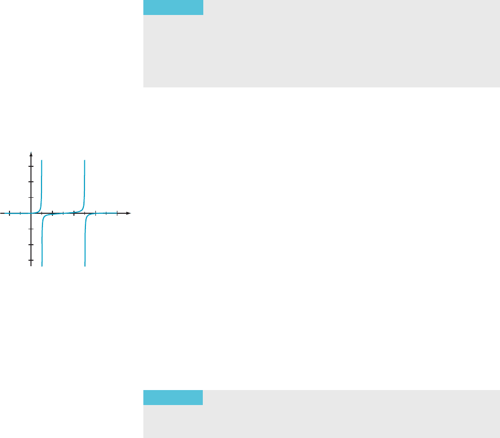
⁄ EX

AMPLE 7 Let FðxÞ5 sinðxÞ; GðxÞ5 x

2 6x 1 5, and HðxÞ5 FðxÞ=GðxÞ:

For which values of x is H continuous?

Solution As

was mentioned earlier in this section, the limit theorems from Section

2.2 tell us that trigonometric functions and polynom ials are continuous. In

particular, the functions F and G are continuous at every point of the real line.

Therefore the function H is continuous at every value of x for which

GðxÞ5 x

2 6x 1 5 5 ðx 2 1Þðx 2 5Þ is nonzero. Thus H is continuous at each point

different from 1 an d 5. The points 1 and 5 are not in the domain of H, so we do not

speak about the continuity of H at these points. The plot of H in the viewing

window ½22; 8 3 ½215; 15 (see Figure 15) indicates that H does not have a

continuous extension at the exceptional points.

If the image of a function f is contained in the domain of a function g, then we

may consider the composition ðg

f ÞðxÞ5 g ðf ðxÞÞ. This equation deﬁnes an

operation that consists of ﬁrst applying f a nd then applying g . In general, using the

limits of f and g to calculate the limit of the composite function g

f can be tricky.

Exercises 5557 at the end of this section explore the possibilities. The following

theorem assures us that nothing unexpected happens when both f and g are con-

tinuous: Composition preserves continuity.

THEOREM 2

Suppose the image of a function f is contained in the domain of a

function g.Iff is continuous at c, and g is continuous at f ðcÞ, then the composed

function g

f is continuous at c.

⁄ EX

AMPLE 8 Is x/ cos ðx

1 1Þ continuous at every x?

Solution The

functions f ðxÞ5 x

1 1 and gðxÞ5 cosðxÞ have the entire real line as

their domai n, and they are continuous at each point. Therefore ðg

f ÞðxÞ5

cosðx

1 1Þ is deﬁned for every value of x, and, by Theorem 2, it is continuous at

every x.

Advanced Properties of

Continuous Functions

The next two theorems about continuity depend on a deeper pr operty of the real

numbers—the completeness propert y. When we imagine the real numbers , we are

accustomed to picturing a line (the real number line) that has no gaps in it. The

analytic formulation of this idea is the completeness property of the real numbers.

There are a number of equivalent ways to express the property precisely. One

15

10

5

82 246

y  H(x)

m Figure 15

H (x) 5 sin

(x)/(x

2 6x 1 5)

2.3 Continuity 111

formulation is the nested interval property, which is discussed in Genesis &

Development, Chapter 1. Another is the least upper bound property of the real

numbers—see Genesis & Development, Chapter 2. A third formulation of the

completeness property is discussed in Section 2.6.

Like many theorems in calculus, the two theorems that follow require that we

use the notion of a function f being continuous on a closed interval ½a; b. This

means that f is continuous at every point in the open interval ða; bÞ, f ðxÞ is right-

continuous at a, and f ðxÞ is left-continuous at b. In particular, if f is continuous on

½a; b, then the functional values f ðaÞ and f ð bÞ at the endpoints are the same as the

one-sided limits of f at the endpoints.

THEOREM 3

(The Intermediate Value Theorem). Suppose that f is a con-

tinuous function on the closed interval ½a; b. Suppose further that f ðaÞ 6¼ f ðbÞ.

Then, for any number γ betwee n f ðaÞ and f ðbÞ, there is a number c between a

and b such that f ðcÞ5 γ.

INSIGHT

In simple language, Theorem 3 states that continuous functions do not

skip values. If f is continuous and takes the values α and β, then f takes all the values

between α and β (see Figure 16). In even plainer language, the graph of f does not have

jumps—a jump would correspond to skipped values. This explains why we sometimes say

that a continuous function can be graphed without lifting the pencil from the paper.

Although we now understand this statement to be purely informal, we can use it to guide

our intuition.

⁄ EXAMPLE 9 Is there a point in the interval ð0; 2Þ at which the funct ion

f ðxÞ5 ðx

11Þ

takes the value 10?

Solution Because

it is a polynomial, the function f (x) 5 (x

1 1)

is continuous.

We can easily ﬁnd values a and b such that γ 5 10 is between f (a) and f (b). For

example, if a 5 0, and b 5 2, then f (a) 5 1 , 10 , 81 5 f (b). According to the

Intermediate Value Theorem, we can be sure that there is a number c between 0

and 2 such that f (c) 5 10.

INSIGHT

The Intermediate Value Theorem gives us conditions under which we can

be certain that the equation f ðcÞ5 γ has a solution c. In Example 9, we can actually ﬁnd a

formula for the value c for which f ðcÞ5 γ. With the aid of a little algebra, we obtain

c 5

ﬃﬃﬃﬃﬃﬃﬃﬃﬃﬃﬃﬃﬃﬃﬃﬃﬃ

ﬃﬃﬃﬃﬃ

2 1

C1:2931:::: When we use the Intermediate Value Theorem, we usually

cannot ﬁnd an explicit formula for the value of a solution c of the equation fðcÞ5 γ: In

Chapter 4, we will learn how to ﬁnd good approximations to the solutions of such

equations.

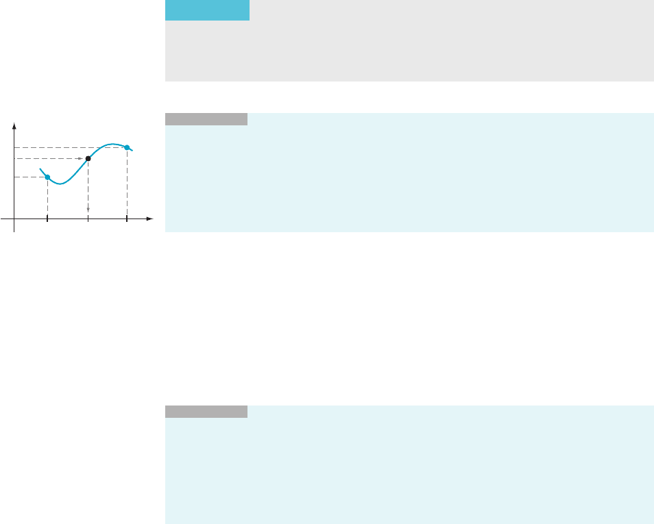
⁄ EXAMPLE 10 Mr. Woodman weighs 150 pounds at noon on January 1

(t 5 1), 130 pounds at noon on January 15 (t 5 15), and 140 pounds at noon on

January 30 (t 5 30). His weight is a continuous function of time t. How often during

the month of January can we be sure that he will weigh 132 pounds?

bac

y  f (x)

 f (b)

a  f (a)

m Figure 16

112 Chapter

2 Limits

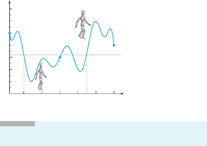
Solution Let w(t) be Mr. Woodman’s weight in pounds at time t where t is

measured in days. Our hypotheses may be written as

wð1Þ5 150; wð15Þ5 130; wð30Þ5 140:

Because 132 is between 150 and 130, there is a time t

,1, t

, 15, such that

wðt

Þ5 132. Likewise, 132 is between 130 and 140. Thus there is a time t

15 , t

, 30, such that wðt

Þ5 132. In other words, we have found that between

noon on January 1 and noon on January 30, Mr. Woodman will weigh 132 pounds

at least two times. As Figure 17 illustrates, Mr. Woodman may weigh 132 pounds at

other times between January 1 and January 30. Without further information,

however, we can only say for certain that there are at least two times.

INSIGHT

As Example 10 illustrates, the Intermediate Value Theorem says nothing

about uniqueness. It gives us conditions under which there is sure to be a solution c of the

equation f (c) 5 γ, but it does not tell whether there is only one solution or several solutions.

We have already mentioned that, if n is a positive integer, then x /

ﬃﬃﬃ

is a

continuous function (Theorem 4 from Section 2.2). Until now, we have implicitly

assumed the existence of nth roots. How can we be sure, however, that there is a

number c such that c

5 π? The Intermediate Value Theorem can be used to prove

the existence of such roots, as shown in the next example.

⁄ EX

AMPLE 11 Let γ be a positive number and n a positive integer. Show

that there is a number c such that c

5 γ.

Solution Let f ðxÞ be

deﬁned on ½0; NÞ by f ðxÞ5 x

. We know that f is a continuous

function by Theorem 3 from Section 2.2. Let a 5 0, b 5 γ 1 1, α 5 f ðaÞ, and β 5 f ðbÞ.

Then,

α 5 f ð0Þ5 0 , γ , γ 1 1 , ðγ11Þ

5 f ðbÞ5 β:

The Intermediate Value Theorem tells us that there is a c in ða; bÞ such that f ðcÞ5 γ.

Thus c

5 γ. ¥

w  132

(1, 150)

(30, 140)

30252015101

120

110

100

130

140

150

160

170

(15, 130)

m Figure 17

2.3 Continuity 113

The Intermediate Value Theorem is said to be an existence theorem because it

asserts the existence of a value without specifying it. We will encounter several

theorems of this type in our study of calculus. Indeed, the theorem that follows

asserts the existence of a highest and a lowest point on the graph of a function that

is continuous on a closed, bounded interval.

DEFINITION

Suppose that f is a function with domain S. If there is a point α in

S such that f ð αÞ # f ðxÞ for all x in S, then the point α is called a minimu m for

the function f, and m 5 f ðαÞ is called the minimum value of f. If there is a point

β in S such that f ðβÞ$ f ðxÞ for all x in S, then the point β is called a maximum

for the function f, and M 5 f ðβÞ is called its maximum value.

THEOREM 4

(The Extreme Value Theorem). If f is a continuou s function on the

closed interval [a, b], then f has a minimum α in [a, b] and a maximum β in [a, b].

INSIGHT

A continuous function on a closed interval [a, b] has a greatest value f ðβÞ

and a least value f ðαÞ. These values are also known as extreme values, or extrema, of f.

⁄ EXAMPLE 12 Let f ðxÞ5 x

2 7x

1 3x 2 1on½0; 4. Does f take a max-

imum value on this interval? Does f take a minimum value?

Solution Because f is

continuous (it is a polynomial), it takes a greatest value at

some point β in ½0; 4 and a least value at some point α in ½0; 4 . We can be sure

that this is true by Theorem 4, even though we do not yet know how to ﬁnd α

and β.

INSIGHT

One important application of calculus is to actually ﬁnd α and β. This, in

turn, will enable us to solve many interesting problems. (Chapter 4 covers this idea in

more detail.)

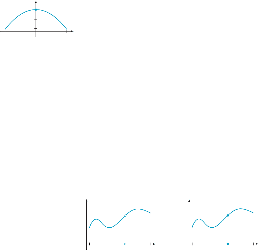
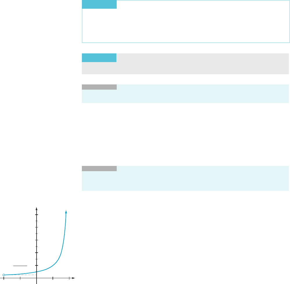
⁄ EXAMPLE 13 Let f ðxÞ5 1=ð1 2 xÞ (see Figure 18). Are there maximum

and minimum values for f on the interval ð21; 1Þ?

Solution Here

the function f is continuous, and the interval ð21; 1Þ is bounded.

However, this interval is not closed because it does not contain its endpoints.

Because the Extreme Value Theorem may only be applied to closed intervals, we

may not use it here. Instead, we must investigate the behavior of f. We observe that

f has no greatest value on the interval ð21; 1Þ because f ðxÞ becomes large without

bound as x approaches 1 from the left (e.g., f ð0:9Þ5 10, f ð0:9999Þ5 10000, etc.).

Also, f has no least value on ð21; 1Þ, although this is so for a more subtle reason—if

x is near 21 and to the right of 21; then f ðxÞ is nearly 1/2. Indeed, the values of

f become arbitrarily close to 1/2 when x is sufﬁciently close to 21 on the right,

but f never actually assumes the value 1/2 at any point of the interval ð21 ; 1Þ. So, f

does not assume a minimum value on ð21; 1Þ.

1 0.5 10.5



(x) 

(x  1)

m Figure 18

114 Chapter

2 Limits