Barber J.R. Intermediate Mechanics of Materials

Подождите немного. Документ загружается.

9.4 The governing equation 425

The attentive reader should immediately recognize this equation as having the

same form as equation (7.5) for the bending of a beam on an elastic foundation. To

understand the reason for this similarity, it might be helpful to regard the shell as a

set of strips, as shown in Figure 9.5. Each strip can be considered as an elastic beam

whose displacement in the radial direction is opposed by the elastic action of the

circumferential stress

All of the solution methods

developed in Chapter 7 can be applied to the solution

of equation (9.20). However, the most important conclusion to be drawn from this

equation, as in §7.3, is that the displacement due to radial loading of the shell will be

localized, decaying exponentially with distance from the load. As before, we deﬁne

a characteristic decay length

= C

√

at , (9.22)

where the numerical factor

C =

3(1 −

)

(9.23)

lies in the very restricted range 0.76<C<0.82 for 0<

<0.5. Thus, the characteristic

length is signiﬁcantly smaller than the radius a, since t ≪a. As an example, a steel

shell of radius 1 m and wall thickness 10 mm will have a characteristic length of 55

mm.

It follows that all practical shells are ‘long’ in the sense of Chapter 7 and can

therefore be analyzed using the inﬁnite or semi-inﬁnite solutions of §§7.4, 7.2.1.

An alternative form for the right hand side of equation (9.20) can be obtained by

noting that the membrane theory predicts that the circumferential stress

= pa/t

for the cylinder and hence the predicted membrane displacement is

(

−

νσ

−

νσ

using (8.5). We can substitute this result into (9.20), obtaining

+ 4

= 4

. (9.24)

This shows that the membrane solution (8.5) gives the exact value for the radial

displacement

as long as the loading is a polynomial of third degree or below in z.

Readers who have not studied Chapter 7 will ﬁnd it helpful to review §§7.2–7.5 in parallel

with the present derivations.

A similar result holds for a beam on an elastic foundation subjected to polynomial loading

and corresponds to the case where u=w(z)/k and the loading is transmitted directly to the

foundation.

426 9 Axisymmetric Bending of Cylindrical Shells

9.4.1 Solution strategy

The ﬁrst stage in the analysis of any axisymmetric shell is to ﬁnd the ‘membrane so-

lution’, using the methods of Chapter 8. We can then identify the regions of the shell

(typically the ends of the shell or discontinuities of radius, thickness or loading) at

which the membrane theory predicts discontinuities of radial displacement or slope.

The bending theory is then used to construct a local solution, treating the shell as

inﬁnite or semi-inﬁnite.

The equilibrium equation used to determine the meridional membrane stress

is unaffected by the presence of local bending, so this value carries over into the

bending calculation. By contrast, equation (8.2) is modiﬁed by the presence of shear

forces [see equation (9.15) above] and hence the circumferential stress

gener-

ally deviates from the value predicted by the membrane theory in a region of local

bending. However, once

is determined, we can solve (9.20) or (9.24) for u

with

appropriate end conditions. The local value of

can then be recovered from equa-

tion (9.17).

It is convenient to summarize these steps as follows:-

(i) Find the axial membrane stress

as in §8.1 by making a cut perpendicular to

the axis, writing an equilibrium equation, and summing forces along the axis.

(ii) Use this result and the internal pressure p to determine the right-hand side of

equation (9.20), which may be a function of z.

(iii) Use the techniques of Chapter 7 to obtain the general solution of equation

(9.20), noting that for uniform or low order polynomials we can ﬁnd a sim-

ple particular solution and that the homogeneous solution is deﬁned by equa-

tion (7.11) or (7.12). Usually the shell can be considered semi-inﬁnite, so we

only need the exponentially decaying terms and these can be written in the form

(7.18).

(iv) Find the constants from the end conditions, using (9.13, 9.19) if necessary to

convert force or moment end conditions to conditions on u

(v) Once u

is known,

can be determined from (9.17).

(vi) The bending moment M

is given by (9.13) and the maximum stresses are then

given by

max

;

max

. (9.25)

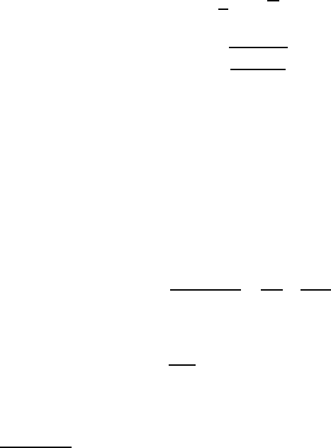
Example 9. 1

A cylindrical steel tube of mean diameter 50 mm and wall thickness 4 mm is built in

to a rigid wall at one end and loaded by an axial force of 60 kN, as shown in Figure

9.6. Find the maximum tensile stress in the tube. There is no internal pressure and

the elastic properties for steel are E =210 GPa,

=0.3.

The axial load of 60 kN will produce a meridional stress

given by the equilib-

rium equation

×50 ×4 ×

= 60 ×10

9.4 The governing equation 427

and hence

60 ×10

×50 ×4

= 95.5 MPa .

Figure 9.6

The membrane solution gives

= 0, from equation (8.2), since there is no in-

ternal pressure and R

= ∞ for the cylinder. Thus the membrane radial displacement

will be

= −

νσ

= −

0.3 ×95.5 ×10

×0.025

210 ×10

= −3.41 ×10

−6

m .

The negative sign indicates that the displacement is radially inwards — the diameter

of the tube gets smaller as a result of Poisson’s ratio strains.

This radial displacement is prevented at the built-in support, where u

= 0 and

/dz= 0. There will therefore be a region of local bending.

We ﬁrst calculate

3(1 −

)

3 ×0.91

×4

= 0.129 mm

−1

(129 m

−1

) ,

corresponding to a characteristic length, l

=7.78 mm.

The membrane displacement u

is constant (independent of z) and hence a suit-

able particular integral of equation (9.24) is u

= u

. A sufﬁciently general solution

of this equation can therefore be written

= u

+ B

(

z) + B

(

z) ,

using equation (7.18) from §7.2 for the homogeneous solution. The corresponding

derivative is

(z) ≡

= −B

(

z) + B

(

z) ,

4 mm

50 mm

60 kN

428 9 Axisymmetric Bending of Cylindrical Shells

from (7.19) and the boundary conditions u

=du

/dz= 0 therefore require that

= −u

; −B

+ B

= 0 ,

with solution

= B

= 3.41 ×10

−6

m .

The bending moment M

is given by equation (9.13, 7.23) as

= −D

= −2D

(

z) −B

(

z)] ,

where

D =

12(1 −

)

210 ×10

×4

×10

−9

12 ×0.91

= 1230 Nm .

The maximum value of M

occurs at z=0 and is

max

= 2D

= 2 ×1230 ×129

×3.41 ×10

−6

= 138.6 Nm per m .

The corresponding maximum bending stress is

max

6 ×138.6

= 52.0 MPa.

This stress is additive to the membrane stress

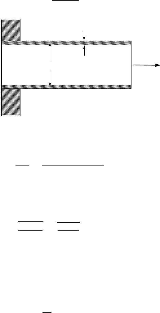
=95.5 MPa. The deformed shape

of the tube is as shown in Figure 9.7, from which we conclude that the maximum

tensile stress (the most extended ﬁbres) occur at the outside of the shell near z = 0,

since this is the outer radius of the curvature in the cross-sectional view. At this point,

we have

= 95.5 + 52.0 = 147.5 MPa .

Alternatively, we can use equation (9.5) to obtain

noting that M

is positive, to determine the maximum stress to be at

=t/2, where

= 95.5 +

12 ×138.6 ×2

= 147.5 MPa .

60 kN

maximum tensile stress

Figure 9.7: Deformed shape of the tube

9.5 Localized loading of the shell 429

A bending moment M

will also be induced in the circumferential direction and

in some situations this can deﬁne the maximum tensile stress, when combined with a

substantial circumferential membrane stress

. We ﬁrst calculate

, using equation

(9.17). At the support, u

=0 and we have

νσ

= 0.3 ×95.5 = 28.7 MPa .

The circumferential bending moment at the support is found from equation (9.8) as

max

= 0.3 ×138.6 = 41.6 Nm per m

and hence

max

θθ

= 28.7 +

6 ×41.6

= 44.3 MPa .

Once again, the maximum occurs at the outer surface of the shell, but it is smaller

than

max

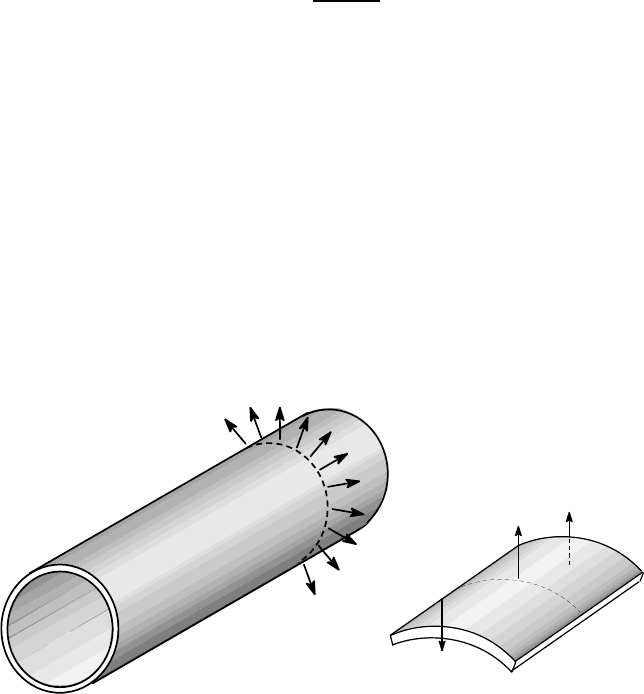
9.5 Locali zed loading of the shell

Figure 9.8 (a) shows a cylindrical shell subjected to an axisymmetric radial load,

per unit circumference. This problem is exactly analogous to the inﬁnite beam

problem of §7.4 and we conclude by analogy with equation (7.35) that the radial

displacement will be given by

(

|z|) , (9.26)

where

is the displacement under the load.

F per unit circumference

F a δθ

V(0 ) a δθ

(a) (b)

Figure 9.8: (a) Cylindrical shell subjected to an axisymmetric radial load; (b) Equi-

librium of a shell element

430 9 Axisymmetric Bending of Cylindrical Shells

To ﬁnd the relation between F

and

, we note that

V = −D

= −4D

δβ

(

|z|)sgn(z) ,

from equations (9.19, 9.26, 7.23), where sgn(z)=1 for z>0 and −1 for z <0. Figure

9.8 (b) shows a small element of shell including the load F

and we conclude that

= −V (0+) +V(0−) = 8

which permits us to rewrite (9.26) in the form

(

|z|) . (9.27)

The corresponding axial bending moment, M

= −D

(

|z|) . (9.28)

As in §7.4.1, we can generalize these results by superposition to obtain the solu-

tion for an arbitrary axisymmetric load acting over the segment a< z <b. We obtain

p(z

′

) f

(

|z −z

′

|)dz

′

(9.29)

p(z

′

) f

(

|z −z

′

|)dz

′

, (9.30)

where we note that a distributed axisymmetric load is equivalent to an internal pres-

sure p that is a function of the axial coordinate z

′

9.6 Shell transition regions

One of the most important applications of the shell bending theory concerns the

design of transitions between different shell segments. We saw in §8.5.1 that the

membrane theory predicts a discontinuity in radial displacement u

whenever there

is a discontinuity in the radius R

, and the reconciliation of this discontinuity always

involves local bending.

Strictly speaking, the theory developed in this chapter applies only to cylindri-

cal shells and hence can only be used for the cylindrical segment, for example, in

the cylinder/sphere transition of Figures 8.21, 8.22. There is a distinct and rather

more complicated theory for the bending of spherical shells.

The results are broadly

similar to those for the cylinder (bending effects are localized and decay away from

the loaded region), but the functions are affected by the fact that the shell becomes

See for example, S.P. Timoshenko and S. Woinowsky-Krieger (1959), Theory of Plates and

Shells, McGraw-Hill, New York, 2nd edn., §§129–132.

9.6 Shell transition regions 431

locally inclined to the axis and has a cross-sectional radius r, which varies with dis-

tance from the loaded region.

However, we have seen that shell bending effects are extremely localized near

the discontinuity and in many cases these complicating factors do not reach signif-

icant proportions within the decay length, permitting the cylindrical shell bending

theory to be used as an approximation. The appropriateness of this approximation

can be assessed by calculating the characteristic length from equation (9.22) and de-

termining the change in radius and shell inclination at the end of the bending zone.

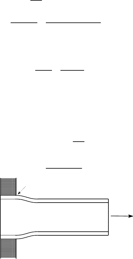
For example, Figure 9.9 shows a toroidal shell segment connecting a cylinder and a

cone. The decay length in the cylinder is

= 0.78

√

at = 0.78

√

500 ×10 = 55 mm .

The region affected by bending is therefore of the order of 55 mm to each side of the

transition between the cylindrical and toroidal segments. On the toroidal side, the

angle subtended at the centre O

is therefore

100

= 0.55 radians = 31.6

and the change in cross-sectional radius, r in this range is

100(1 −cos31.6

) = 14.8 mm .

Thus, in this region, the toroidal segment is sufﬁciently close to a cylinder to justify

the use of the cylindrical bending theory, at least to obtain a ﬁrst approximation to

the magnitude of the bending stresses.

500 mm

100 mm

10 mm

Figure 9.9: Transition from a cylinder to a toroidal shell segment

To determine the bending stresses associated with a transition between two shell

segments, we ﬁrst calculate the membrane stresses and displacements to determine

the discontinuity in u

predicted at the transition. The reconciliation of this disconti-

nuity is then effected by applying equal and opposite forces and moments to the two

segments, as in Example 7.3. As in that case, the maximum bending moment occurs

at the two points

z= ±

/4.

432 9 Axisymmetric Bending of Cylindrical Shells

Example 9. 2

Find the maximum tensile and compressive stresses for the toroidal to cylindrical

transition of Figure 9.9, if the internal pressure is 2 MPa.

We ﬁrst calculate the membrane stresses and displacements. For both toroidal

and cylindrical segments at the transition, we have

p ×

2 ×500

2 ×10

= 50 MPa .

For the cylinder,

2 ×500

= 100 MPa ,

whereas for the toroidal segment (R

=100 mm, R

=500 mm),

= R



−



= 500



−

100



= −150 MPa .

The membrane displacements are

(

−

νσ

(100 −0.3 ×50)500

210 ×10

= 0.202 mm (cylinder)

(−150 −0.3 ×50)500

210 ×10

= −0.393 mm (toroidal segment) .

The bending solution must therefore reconcile a discontinuity

=0.202+0.393=

0.595 mm in u

, half of which will be accommodated on each side of the transition.

The bending moment will be zero at the transition and hence the bending displace-

ment will be

(

z) ,

by analogy with equation (7.24), where

= 1/l

= 18.2 m

−1

(the value of l

= 55

mm was calculated above). The stiffness of the shell is

D =

12(1 −

)

210 ×10

×10

−9

12 ×0.91

= 19,230 Nm

and the axial bending moment is therefore

= −D

δβ

(

z) .

The maximum value of this expression occurs at

/4 and is

max

= 0.322D

δβ

= 0.322 ×19,230 ×0.595 ×10

−3

×18.2

= 1258 Nm per m .

The corresponding maximum bending stress is

9.6 Shell transition regions 433

max

6 ×1258

= 75.5 MPa ,

giving a maximum axial stress

max

= 50 + 75.5 = 125.5 MPa .

We should also check to ensure that the circumferential stress

θθ

nowhere ex-

ceeds this maximum value. We recall that the circumferential membrane stress

νσ

from equation (9.17). For most of the shell, this will be lower than the limiting value

of 100 MPa in the cylindrical segment, since the transition restrains the shell from ex-

pansion. However, the oscillatory nature of the decaying function f

(x) ensures that

there is an axial location at which u

> u

and hence

> 100 MPa. The maximum

will occur where

(z) =

β δ

(

z) = 0

and hence cos(

z)+sin(

z) = 0. The ﬁrst solution of this equation is at

z = 3

/4,

where

= −





= −

0.595 ×(− 0.067)

= 0.020 mm .

We therefore have,

max

210 ×10

(0.202 + 0.020)

500

+ 0.3 ×50 = 108.2 MPa .

In addition, the circumferential bending moment at this point is

νβ

D f





= 0.3×19,230×0.595×10

−3

×18.2

×0.067 = 76 Nm per m ,

contributing an additional stress

θθ

6 ×76

= 4.6 MPa .

However, it is clear that the maximum tensile stress in the shell is the axial stress

max

=125 MPa.

9.6.1 The cy linder/cone transition

The toroidal shell of Example 9.2 is often used to form a transition between a cylin-

drical and a conical shell segment, as shown in Figure 9.10. In this section, we shall

discuss the criteria that might be used to determine an appropriate transition radius,

434 9 Axisymmetric Bending of Cylindrical Shells

Figure 9.10: Toroidal transition from a cylinder to a cone

If R is small, the circumferential membrane stress

will be negative (compres-

sive) in the toroidal segment and the displacement discontinuity

to be reconciled

by bending will be relatively large. In this case, the largest tensile stress in the shell

will be the axial stress

, as in Example 9.2, and it will be dominated by the bending

term 6M

Increasing R will reduce the bending stresses, but the total stress cannot be lower

than the membrane stresses

and these are dominated by the circumferential

stress

in the cylindrical and conical segments. Thus, there is nothing to be gained

by increasing R beyond the point at which the maximum total axial stress is equal

to the largest value of

. Depending on the semi-angle of the cone, this break-even

point occurs in the range R/a= 0.5 ∼0.6 (see Problem 9.7).

cone

cylinder

cone

cylinder

(a) (b) (c)

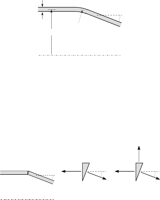
Figure 9.11: (a) Abrupt cylinder/cone transition; (b) loading of the connecting ele-

ment; (c) Equilibrium restored by a radial force

At the other extreme, we could make an abrupt transition from the cylinder to the

cone, as shown in Figure 9.11 (a). In this case, the small triangular element connect-

ing the segments will be subject to the loading shown in Figure 9.11 (b) and it cannot

be in equilibrium. The meridional stresses are calculated in the usual way as