Barber J.R. Intermediate Mechanics of Materials

Подождите немного. Документ загружается.

3.6 The Rayleigh-Ritz method 125

where n is an integer, obtaining

U =

∑

i=1

The potential energy of the load is

Ω

w(z)u(z)dz , (3.54)

where u(z) is assumed to be positive upwards. The total potential energy is

= U +

Ω

∑

i=1

∑

i=1

w(z)sin





dz .

Finally, we can ﬁnd the coefﬁcients C

from the conditions

∂Π

∂

= 0 =

EIi

w(z)sin





dz ; i = (1,N)

and hence

= −

EIi

w(z)sin





dz . (3.55)

This result is remarkable in that the coefﬁcients C

are obtained explicitly, with-

out the need to solve a system of N simultaneous equations. This is a consequence of

the orthogonality of the trigonometric functions (3.53), which causes all the integrals

in U to be zero except those where i = j. For this reason, it is possible to allow the

number of terms N to increase without limit and hence obtain an exact solution for

the problem of the simply-supported beam with arbitrary loading w(z). This tech-

nique can also be used for other categories of problem, such as a rectangular plate

simply-supported around its edges

and a rectangular plate subjected to in-plane

Finite element solutions

A series approximation consists of a denumerable set of linearly independent func-

tions, each of which is deﬁned over the entire length of the beam. An alternative

approach is to use a discrete approximation — i.e. to split the beam into a number of

segments and use an independent low order approximation to the deﬂection in each

segment. The combination of a discrete approximation to the deﬂection and the use

of a variational principle (such as the stationary potential energy theorem) to choose

S.P. Timoshenko and S. Woinowsky-Krieger (1959), Theory of Plates and Shells, McGraw-

Hill, New York, §80.

S.P. Timoshenko and J.N. Goodier (1970), Theory of Elasticity, Mc-Graw-Hill, New York,

§94.

126 3 Energy Methods

the ‘best’ values of the resulting degrees of freedom is known as the ﬁnite element

method.

For relatively small numbers of degrees of freedom (say less than 10), there is

little to choose between the two methods, but series methods become progressively

more inaccurate due to rounding errors when large numbers of terms are used and

the discrete method is therefore to be preferred for solutions of high accuracy.

The ﬁnite element method is an extremely important tool in modern mechanics

of materials. It is therefore discussed in more depth in Appendix A.

3.6.2 Improving the back of the envelope approximation

Series and discrete approximations are useful ways of developing a relatively accu-

rate approximation to a problem, but they generally involve susbtantial analytical or

numerical work. We have already seen how a simple one term approximation can

give estimates for deﬂection that are within 50% of the exact value with only a few

lines of calculation. Fortunately, this ‘back of the envelope’ estimate can often be

improved without adding extra degrees of freedom and hence with only a limited

amount of additional calculation.

The solution is approximate only because we are seeking it within a restricted

class of trial functions. The accuracy can therefore be improved if we can make

use of additional information about the structure to choose a better approximating

function. This information may be based on our knowledge of mechanics, or it may

be more or less intuitive. We shall give examples of both kinds in this section.

Example 3. 7 revisited

As an example of the ﬁrst approach, we note that the bending moment is zero at

z = L in Example 3.7 so that the curvature there (d

u/dz

) must be zero. The form

assumed in equation (3.47) clearly does not satisfy this condition, since its second

derivative is constant — in other words the curvature is constant along the beam.

We would therefore expect to get a better result if we chose a form that deﬁned

zero curvature at z=L for all values of the constant C. We could develop such a form

by starting with a polynomial of two-degrees of freedom — for example

u = C

(3.56)

and then choosing the second constant C

to satisfy the condition. Notice that (3.56)

still satisﬁes the essential kinematic support conditions u = du/dz = 0 at z = 0. The

curvature at a general point is

= 2C

+ 6C

and hence it will be zero at z= L if C

=−C

/3L. Substituting this result into (3.56),

we obtain

3.6 The Rayleigh-Ritz method 127

u = C



−



which is a one degree of freedom approximation (there is only one constant C

to de-

termine from the principle of stationary potential energy) that satisﬁes the condition

of zero curvature at z= L.

However, we are not restricted to polynomial forms. Trigonometric functions

also give relatively straightforward algebraic solutions and in the interests of variety,

we shall use the form

u = C

1 −cos



i

, (3.57)

which also has only one degree of freedom (C), satisﬁes the kinematic support con-

ditions u = du/dz = 0 at z = 0, and the additional condition that curvature be zero at

z= L, since

cos





and the argument of the cosine is

/2 when z= L.

Repeating the calculation with this approximate shape, we ﬁnd

U =

EIC





cos





dx =

EIC





cos

64L

, (3.58)

from (3.48, 3.57) where we have used the change of variable

z/2L to evaluate

the integral.

Also,

Ω

= w

1 −cos



i

dz =

2Lw

(1 −cos

= w



1 −



, (3.59)

from equations (3.54, 3.57).

We then have

= U +

Ω

64L

+ w



1 −



and the principle of stationary potential energy gives

∂Π

∂

= 0 =

32L

+ w



1 −



— i.e.

C = −

32w



1 −



= −0.119

128 3 Energy Methods

In particular, the end deﬂection is

= u(L) = C = −0.119

. (3.60)

This improved approximate result is only 5% lower than the exact expression, which

is −0.125w

/EI, from equation (3.50) with z = L. By contrast, the ‘unthinking’

trial function (3.47) underestimated the end deﬂection by 33%. Thus, a careful choice

of approximate form results in this case in a quite respectable approximate solution

for the deﬂection even though it uses only a single degree of freedom.

Physical intuition, as discussed in §1.2.1, can also play an important part in de-

veloping a more appropriate Rayleigh-Ritz approximation. We illustrate this process

with the following example.

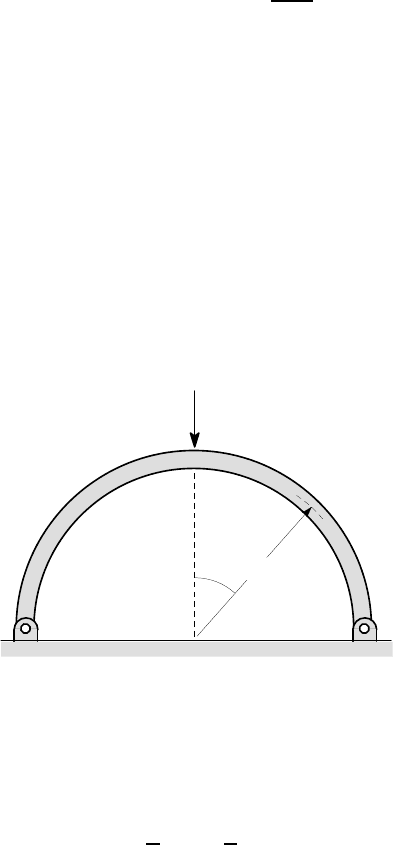
Example 3. 8

A semi-circular curved beam is pinned at its ends and subjected to a concentrated

force F at the mid-point, as shown in Figure 3.18. Estimate the deﬂected shape of

the beam and, in particular, the deﬂection under the load at B.

Figure 3.18: A semi-circular beam subjected to a central load

Deﬁning the outward radial displacement u as a function of angular position

it is clear that the kinematic support conditions require



−



= u





= 0 (3.61)

and a simple one degree of freedom function satisfying these conditions is

u = C cos

. (3.62)

However, this deﬁnes a displacement which has the same sign throughout −

/2 <

/2 and hence corresponds to a mode of deformation like that shown in Figure

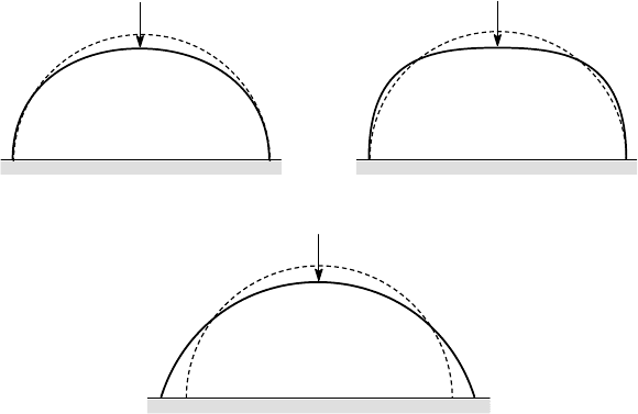
3.6 The Rayleigh-Ritz method 129

3.19 (a), but our intuition tells us that a slender beam will deform instead into the

shape shown in Figure 3.19 (b) — in other words, pushing down in the middle and

restraining the ends will cause the beam to bulge outwards at each side.

(a) (b)

(c)

Figure 3.19: Possible deformation modes for the curved beam

It should be emphasised that people with no training in mechanics have sufﬁcient

intuitive or unconsciously learnt knowledge of the physical world to expect the de-

formation pattern 3.19 (b) rather than 3.19 (a). The reader might like to verify this by

asking their non-technical friends to sketch the deformed shape, without prompting

them with any suggestions. It is of course easily tested by bending a piece of wire

into a semicircle and loading it whilst restraining the ends from horizontal motion

(If the ends are not restrained, the deformation pattern 3.19 (c) will be produced). By

contrast, many engineers will approach the problem in a more formal manner by stat-

ing the boundary conditions (3.61) and will propose the inappropriate form (3.62),

resulting in completely unrealistic estimates for the displacements. The moral here

is “Always sketch the shape you expect the body to adopt, before seeking an appro-

priate approximating function.”

An equally simple form that does look like Figure 3.19 (b) is

u = C cos(3

) (3.63)

since cos(3

) changes sign at the two points

=±

/6.

This function will give a much better approximation to the problem, but we can

do even better, by combining our knowledge of mechanics with our intuition to ask

why the beam deforms into a shape like Figure 3.19 (b). The reason is to be found

in the fact (discussed in §3.3.2 above) that beams are much stiffer in tension than in

bending and hence tend to deform into conﬁgurations that substantially preserve their

130 3 Energy Methods

original length, if any such conﬁguration is kinematically possible. The conﬁguration

3.19 (a) implies that the beam is shorter in the deformed than in the undeformed state.

To a ﬁrst approximation, the deformed length will be

L =

−

(R + u)d

(3.64)

compared with an initial length L

R. Thus, there will be a change in length unless

L = L −L

−

= 0 (3.65)

This in turn requires that there be some regions in −

/2 <

/2 in which u is

positive and some in which it is negative, the simplest such conﬁguration being that

of Figure 3.19 (b).

Now although (3.63) deﬁnes a shape like Figure 3.19 (b), it does not satisfy equa-

tion (3.65) and we should anticipate a signiﬁcantly better approximation if we could

choose a form that does so. As in the previous example, we can develop such a form

by writing the two degree of freedom expression

u = C

cos

cos(3

)

and then choosing C

to satisfy (3.65) with the result C

= 3C

. This deﬁnes the one

degree of freedom approximation

u = C

[cos

+ 3cos(3

)] (3.66)

We shall develop a Rayleigh-Ritz solution to the problem of Figure 3.18, using this

approximating function.

We ﬁrst need to adapt equation (3.48) to the curved beam. The elemental length

of beam dx is replaced by the arc length Rd

, and we might expect the change in

curvature of the beam to be the second derivative of u with respect to the arc length —

i.e. (1/R

u/d

. However, even if u were constant (and hence had no derivative

with respect to

), there would be a change of curvature, since the constant radial

displacement u would change the radius of the beam from R to R + u, resulting in

a reduction in curvature of magnitude u/R to the ﬁrst order. Using these results, the

expression equivalent to (3.48) for the curved beam of Figure 3.18 is

U =

−





, (3.67)

which, after substituting for u from equation (3.66) and evaluating the integral, yields

U =

144

EIC

The potential energy of the force F is simply

3.7 Castigliano’s ﬁrst theorem 131

Ω

= Fu(0) = 4FC

and hence

= U +

Ω

144

EIC

+ 4FC

Applying the principle of stationary potential energy,

∂Π

∂

=0, we obtain

= −

and hence the downward displacement of the force F is

= −u(0) = − 4C

= 0.0177

. (3.68)

This problem can be solved exactly using Castigliano’s second theorem (see be-

low §3.10 and Problem 3.51), the exact solution for u

being

= 0.0189

, (3.69)

so our one degree of freedom Rayleigh-Ritz approximation underestimates the dis-

placement by 7%. By contrast, the result obtained using the superﬁcially plausible

expression (3.63) is 0.00995FR

/EI which is only just over half of the correct an-

swer.

3.7 Casti gliano’s ﬁrst theorem

In this section, we shall introduce a method which is essentially equivalent to the

principle of stationary total potential energy, but which looks at the problem in a

slightly different way.

Suppose we have a complicated elastic system, supported in some way (it can

be determinate or indeterminate) and subjected to N external forces,F

, i = (1,N).

The structure will generally deform under the action of the forces, causing them

to do work which is stored as strain energy. We denote the distance through which

moves in its own direction (i.e. the component of displacement of the point of

application of F

in the direction parallel to F

) by u

Now consider the following scenario:-

(i) The system is ﬁrst allowed to reach its equilibrium conﬁguration under the in-

ﬂuence of the forces F

. Suppose that the strain energy in this state is U.

(ii) All the displacement components u

are then ﬁxed at their equilibrium values,

except one, which we denote by u

(iii) A small additional force dF

is then applied, such that u

increases by du

. There

is no corresponding increase in u

,i 6= k, since these displacement components

are ﬁxed, but additional forces will be induced at the ﬁxed points. After dF

applied the strain energy will generally be changed to U + dU.

132 3 Energy Methods

The system is elastic, so the work done during the incremental loading [stage (iii)

above] must be stored in the structure and is therefore equal to the increase in strain

energy dU . However, the only force that moves during this stage (and hence does

work) is F

, since all the other displacement components are ﬁxed.

The relation

between F

and u

during stage (iii) may be non-linear, as shown in Figure 3.20, but

for sufﬁciently small dF

, the work done (equal to the shaded area under the curve)

can be written

dW = F

= dU .

Figure 3.20: Work done during the application of dF

In fact, if dF

is sufﬁciently small, we can also drop the second term in this

equation, giving in the limit

dU = F

∂

. (3.70)

This result was ﬁrst obtained by Castigliano

and is known as Castigliano’s ﬁrst

theorem. Strictly, following the conventions of thermodynamics, we should write it

in the form



∂



(i6=k)

to indicate that the partial derivative — like the incremental process it describes — is

taking place under the constraint that the remaining points i6=k have zero incremental

displacement.

Castigliano’s ﬁrst theorem is really a restatement of the principle of stationary

potential energy. If we take the undeformed position of the system as the datum for

potential energy of the each of the forces, we have

By the same token, the support reactions do no work either.

A. Castigliano (1879), Th´eory de l‘´equilibre des syst`emes ´elastiques et ses applications,

Turin.

3.7 Castigliano’s ﬁrst theorem 133

Ω

= −F

from equation (3.41), for the potential energy of the force F

and hence

= U +

Ω

= U −

∑

i=1

. (3.71)

Now the principle of stationary potential energy states that

∂Π

∂

= 0

for all k, for small perturbations about the equilibrium position. Substituting for

from (3.71), we recover

∂

−F

= 0 ,

which is identical with (3.70). In effect, the form (3.70) simply eliminates the stage

of writing the total potential energy of the applied forces.

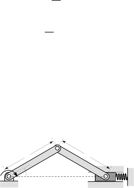
Example 3. 9 — The torque wrench

Figure 3.21 shows an idealization of a torque wrench, designed to permit a nut to be

tightened to a speciﬁc value of torque. The dimensions are deﬁned such that the angle

when the spring is relaxed. If the torque T is increased from zero,

decreases,

but there is a maximum torque at some angle

, beyond which the wrench would

‘snap through’ in an unstable manner to the other side of the horizontal — i.e. to

negative values of

. Determine (i) the relation between the applied torque T and

the angle

and (ii) the maximum value of torque that can be applied without the

mechanism snapping through.

Figure 3.21: The torque wrench

The distance AD is constant and hence the compression u of the spring must be

u = 2Lcos

−2L cos

The strain energy in the spring is therefore

C D

134 3 Energy Methods

U =

(2Lcos

−2L cos

)

and Castigliano’s ﬁrst theorem immediately yields

T = −

∂

∂θ

= 4kL

sin

(cos

−cos

) , (3.72)

which is the required relation between torque and angle of rotation.

Notice that the

only external forces acting are the torque T and the reactions at A,C and D and, of

these, only the torque does any work during the motion, thus meeting the require-

ments of the theorem.

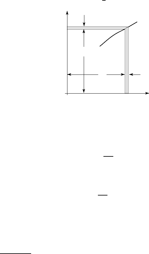
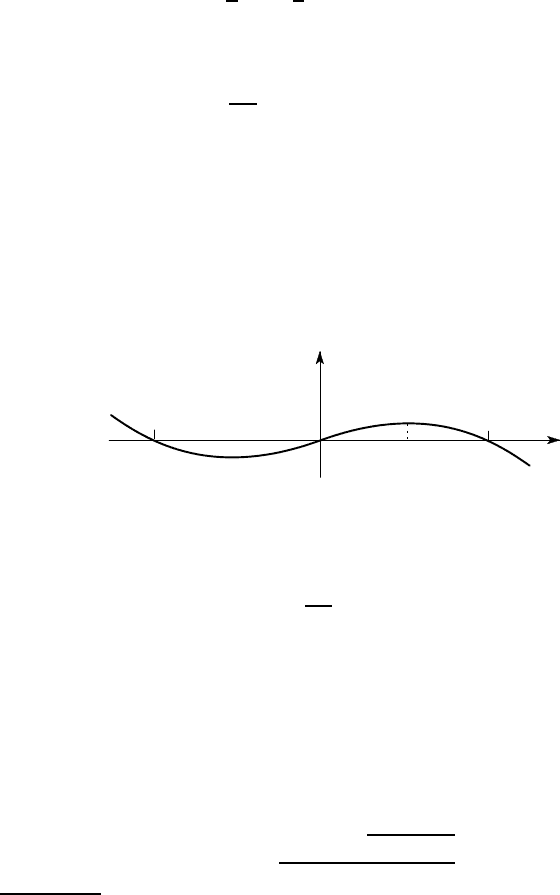
Equation (3.72) is shown graphically in Figure 3.22 and exhibits a maximum

torque in the range 0 <

. If we increase T monotonically,

will fall steadily

until this maximum is reached, when the mechanism will snap through dynamically

to a new equilibrium point beyond

=−

−

Figure 3.22: Relation between torque and rotation for the torque wrench

To ﬁnd the maximum torque, we set

∂

∂θ

= 0

obtaining

cos

(cos

−cos

) + sin

(−sin

) = 0 .

Thus, the critical value

is deﬁned by

2cos

−cos

cos

−1 = 0 ,

where we have used the identity −sin

=cos

−1. The solution of this equation

cos

8 + cos

. (3.73)

The ‘direct’ method of solving this problem would be to draw a free-body diagram of the

system, write equilibrium equations for the separate components to determine the reactions

and internal forces and ﬁnally relate the force in the spring to its deformed length and hence

to the angle

through the kinematics of the mechanism. The reader might like to begin the

solution of the problem by this method. It will rapidly become apparent that this is a case

where the energy method is considerably more efﬁcient.