Atkinson K. An Introduction to Numerical Analysis
Подождите немного. Документ загружается.

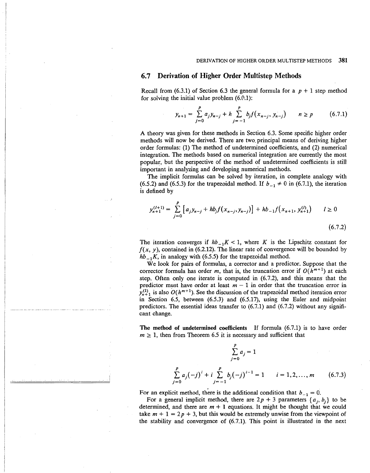
DERIVATION OF HIGHER ORDER MULTISTEP METHODS 381
6.7 Derivation of Higher Order Multistep Methods
Recall from (6.3.1) of Section 6.3 the general formula for a p + 1 step method
for solving the initial value problem
(6.{\.1):
p p
Yn+1
= L ajYn-j + h L
bjf(xn-j•
Yn-j)
n~p
(6.7.1)
j=O
j-
-1
A theory was given for these methods in Section 6.3. Some specific higher
order
methods will now be derived. There are two. principal means
of
deriving higher
order
formulas: (1) The method
of
undetermined coefficients, and (2) numerical
integration.
The
methods based
on
numerical integration
are
currently the most
popular,
but
the perspective
of
the method
of
undetermined coefficients is still
important
in analyzing
and
developing numerical methods.
The
implicit formulas
can
be
solved
by
iteration, in complete analogy with
(6.5.2)
and
(6.5.3) for the trapezoidal method.
If
b_
1
-:!=
0
in
(6.7.1), the iteration
is defined
by
p
Y~~+1
1
)
= L [ajYn-j +
hbjf(xn-j•Yn-)]
+ hb_1J(xn+1•
Y~2J
I~
0
j=O
(6.7.2)
The
iteration converges if hb_
1
K < 1, where K
is
the Lipschitz
constant
for
f(x,
y),
contained in (6.2.12).
The
linear rate
of
convergence will be
bounded
by
hb _
1
K, in analogy with (6.5.5) for the trapezoidal method.
We
look for pairs of formulas, a corrector
and
a predictor. Suppose
that
the
corrector formula has order
m, that is, the truncation
error
if
0(
hm+
1
)
at
each
step. Often only one iterate is computed in (6.7.2),
and
this means
that
the
predictor must have order
at
least m - 1 in
order
that
the
truncation
error
in
y~~
1
is also O(hm+
1
).
See
the
discussion of the trapezoidal method iteration
error
in Section 6.5, between (6.5.3)
and
(6.5.17), using the Euler
and
midpoint
predictors.
The
essential ideas transfer to (6.7.1)
and
(6.7.2) without any signifi-
cant
change.
The
method
of
undetennined coefficients
If
formula (6.7.1)
is
to have
order
m
~
1, then from Theorem 6.5 it is necessary
and
sufficient that
p p
"'
(
")
i + .
"'
b (
•)
i-1
1
1.., aj
-1
1 1.., j
-1
=
i =
1,2,
...
, m
(6.7.3)
j=O
j=
-1
For
an
explicit method, there is the additional condition
that
b_
1
=
0.
For
a general implicit method, there are 2 p + 3 parameters
{a
j•
bj}
to
be
determined,
and
there are m + 1 equations.
It
might be thought that we could
take
m + 1 = 2 p +
3,
but
this would be extremely unwise from the viewpoint
of
the
stability
and
convergence
of
(6.7.1). This
point
is illustrated in the next
382 NUMERICAL METHODS FOR ORDINARY DIFFERENTIAL EQUATIONS
section
and
in the problems. Generally, it
is
best to let m s p + 2 for an implicit
method.
For
an explicit method, stability considerations are often not as im-
portant because the method
is
usually a predictor for an implicit formula.
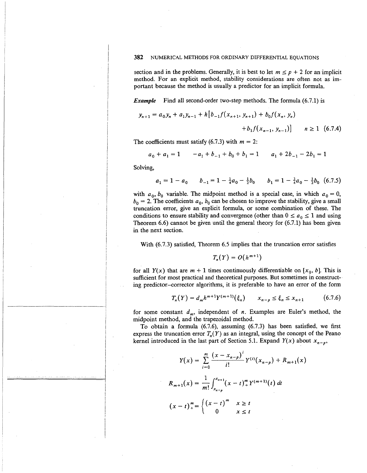
Example Find all second-order two-step methods. The formula (6.7.1)
is
n
~
1 (6.7.4)
The coefficients must satisfy (6.7.3) with m =
2:
Solving,
with
a
0
,
b
0
variable. The midpoint method
is
a special case, in which a
0
=
0,
b
0
=
2.
The
coefficients a
0
,
b
0
can be chosen to improve the stability, give a small
truncation error, give an explicit formula, or some combination of these. The
conditions
to
ensure stability and convergence (other than 0 s a
0
s 1 and using
Theorem
6.6) cannot be
given
until the general theory for (6.7.1) has been given
in the next section.
With
(6.7.3) satisfied, Theorem 6.5 implies that the truncation error satisfies
for all
Y(x)
that are m + 1 times continuously differentiable on [x
0
,
b].
This
is
sufficient for most practical and theoretical purposes. But sometimes in construct-
ing predictor-corrector algorithms, it is preferable to have an error of the form
(6.7.6)
for some constant
dm,
independent of n. Examples are Euler's method, the
midpoint method, and the trapezoidal method.
To
obtain a formula (6.7.6), assuming (6.7.3) has been satisfied,
we
first
express the truncation error
Tn(Y) as an integral, using the concept of the Peano
kernel introduced in the last part of Section 5.1. Expand
Y(x)
about
xn-p•
m (
)i
(
)
"
X-
Xn-p
Cl(
) ( )
y X =
£...-
.,
y I
xn-p
+
Rm+l
X
i=O
l.
(x-t):=
{(x~t)m
x~t
xst
DERIVATION OF HIGHER ORDER MULTISTEP METHODS 383
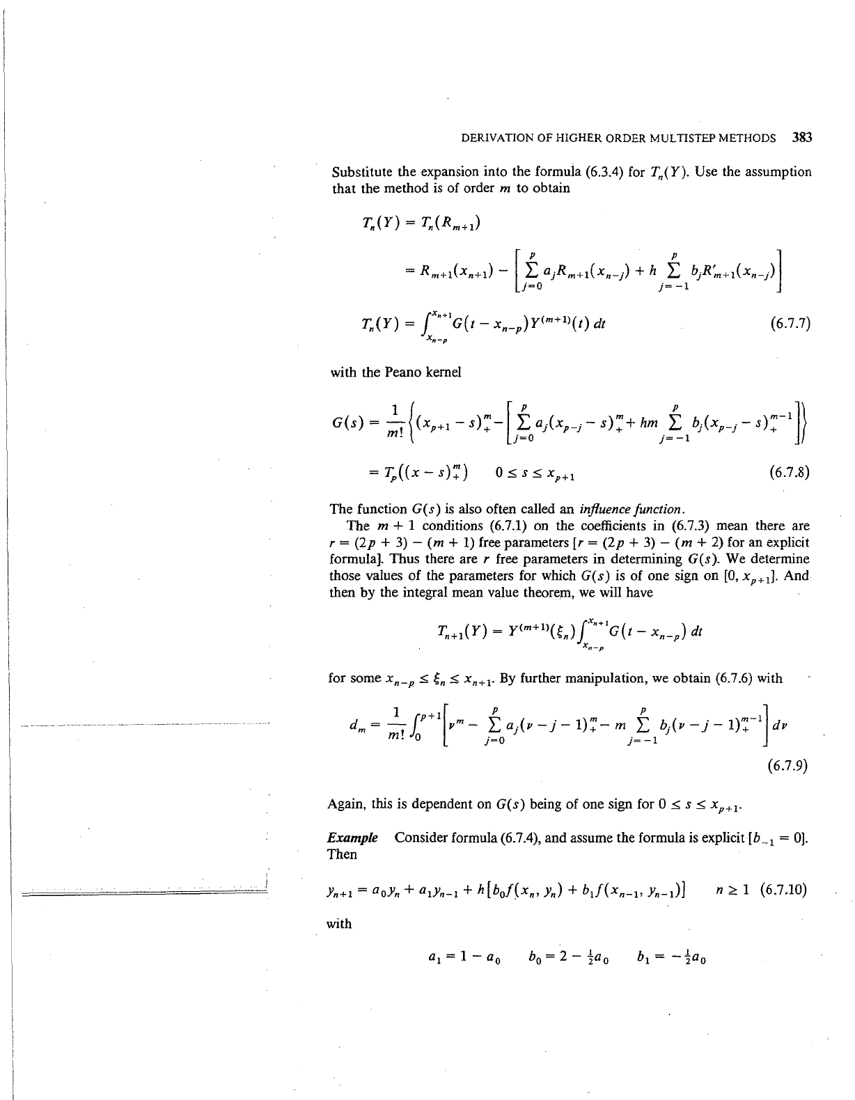
Substitute the expansion into the formula (6.3.4) for
Tn(Y). Use the assumption
that
the
method is of order m to obtain
!
Xn+l
( )
T,(Y) = G
t-
xn-p
y<m+ll(t)
dt
Xn-p
(6.7.7)
with the Peano kernel
(6.7.8)
The
function
G(s)
is also often called
an
influence function.
The
m + 1 conditions (6.7.1) on the coefficients in (6.7.3) mean there are
r =
(2p
+
3)-
(m
+ 1) free parameters
[r
=
(2p
+
3)
-
(m
+ 2) for an explicit
formula].
Thus
there are r free parameters
in
determining
G(s).
We determine
those values
of
the parameters for which
G(s)
is
of
one sign
on
[0,
xp+rl·
And
then
by
the integral mean value theorem, we will have
T,+l(Y) =
y<m+ll(gn)
jx•+lG(t-
xn-p)
dt
Xn-p
for some
xn-p
,:5;
~n
,:5;
xn+I·
By further manipulation, we obtain (6.7.6) with
dm
=
-,lp+l
Pm-
L
a/v-
j-
1)7-
m L
bj(v-
j-
1)':-
1
dv
1 [ p p l
m.
o
j=O
j=-1
(6.7.9)
Again, this is dependent on
G(s)
being of one sign for 0
,:5;
s
,:5;
xp+
1
•
Example Consider formula (6.7.4), and assume the formula is explicit[b _
1
=
0].
Then
n;::::
1 (6.7.10)
with
b
0
=
2-
~a
0
!
i
I
i
---·-----------··-··--------··--·-·--·-·-·-··!
384
NUMERICAL
METHODS FOR ORDINARY DIFFERENTIAL EQUATIONS
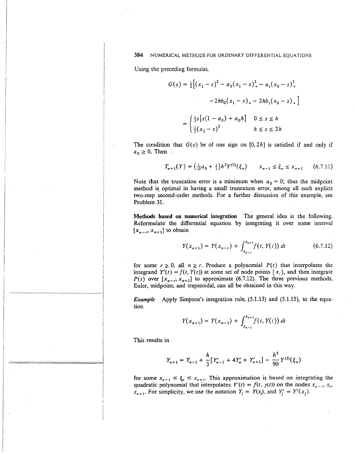
Using the preceding formulas,
= J
!s[s(l-
a
0
)
+ a
0
h]
\Hx
2
-s)
2
O::;s::;h
h
::;
s
::;
2h
The
condition that
G(s)
be of one sign
on
[0,
2h]
is
satisfied if and only if
a
0
~
0.
Then
.
(6.7.11)
Note
that
the truncation error
is
a minimum when a
0
=
0;
thus the midpoint
method
is.
optimal in having a small truncation error, among all such explicit
two-step second-order methods.
For
a further discussion
of
this example, see
Problem 31.
Methods based on numerical integration The general idea is the following.
Reformulate· the differential equation by integrating it over some interval
[x,_,,
x,+
1
]
to obtain
Y(x,+
1
)
=
Y(x,_,)
+ jx""'"'j(t,
Y(t))
dt
xn-r
(6.7.12)
for some r
~
0,
all n
~
r.
Produce a polynomial
P(t)
that interpolates the
integrand
Y'(t)
=
f(t,
Y(t))
at some set
of
node points {x;},
and
then integrate
P(t)
over [x,_,·,
x,+d
to approximate (6.7.12). The three previous methods,
Euler, midpoint, and trapezoidal, can all
be
obtained in this way.
Example Apply Simpson's integration rule, (5.1.13) and (5.1.15), to the equa-
tion
Y(x,+l) = Y(x,_
1
)
+
jx•+'j(t,
Y(t))
dt
Xrr-1
This results in
for some x,._
1
~
~~~
~
x,.+
1
•
This approximation
is
based
on
i~tegrating
the
quadratic polynomial that interpolates Y'(t) =
f(t,
y(t))
on
the nodes
x,
_,,
x,.
x,.+
1
•
For
simplicity, we use the notation
lj
= Y(x), and
~·
=
Y'(x).
DERIVATION OF HIGHER ORDER MULTISTEP METHODS 385
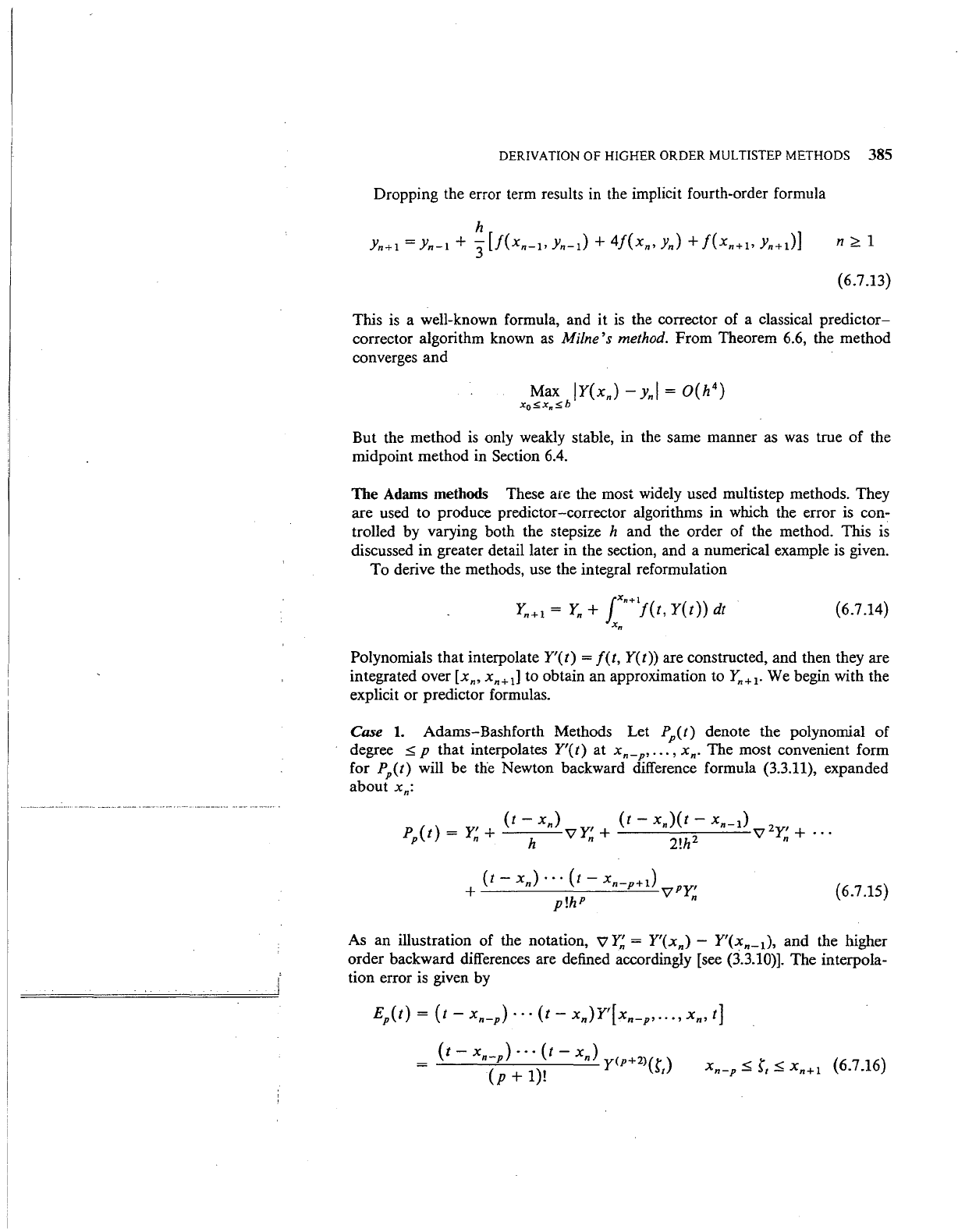
Dropping the error term results in the implicit fourth-order formula
h
Yn+l
= Yn-1 + 3
[f(xn-1•
Yn-1)
+
4f(xn,
yJ
+ f(xn+1• Yn+l)]
n;;:::,
1
(6.7.13)
This is a well-known formula, and it is the corrector of a classical
predictor-
corrector algorithm known as Milne's method.
From
Theorem 6.6, the method
converges
and
But the method is only weakly stable, in the same manner as was true
of
the
midpoint method in Section 6.4.
The
Adams methods These are the most widely used multistep methods. They
are used
to
produce predictor-corrector algorithms
in
which the error is con-
trolled by varying both the stepsize h
and
the order
of
the method. This is
discussed
in
greater detail later
in
the section, and a numerical example is given.
To
derive the methods, use the integral reformulation
f
Xn+l
Yn+l
=
Yn
+
J(t,
Y(t))
dt
x.
(6.7.14)
Polynomials
that
interpolate
Y'(t)
=
f(t,
Y(t)) are constructed, and then they are
integrated over [xn, xn+d to obtain
an
approximation to
Yn+I·
We begin with the
explicit
or
predictor formulas.
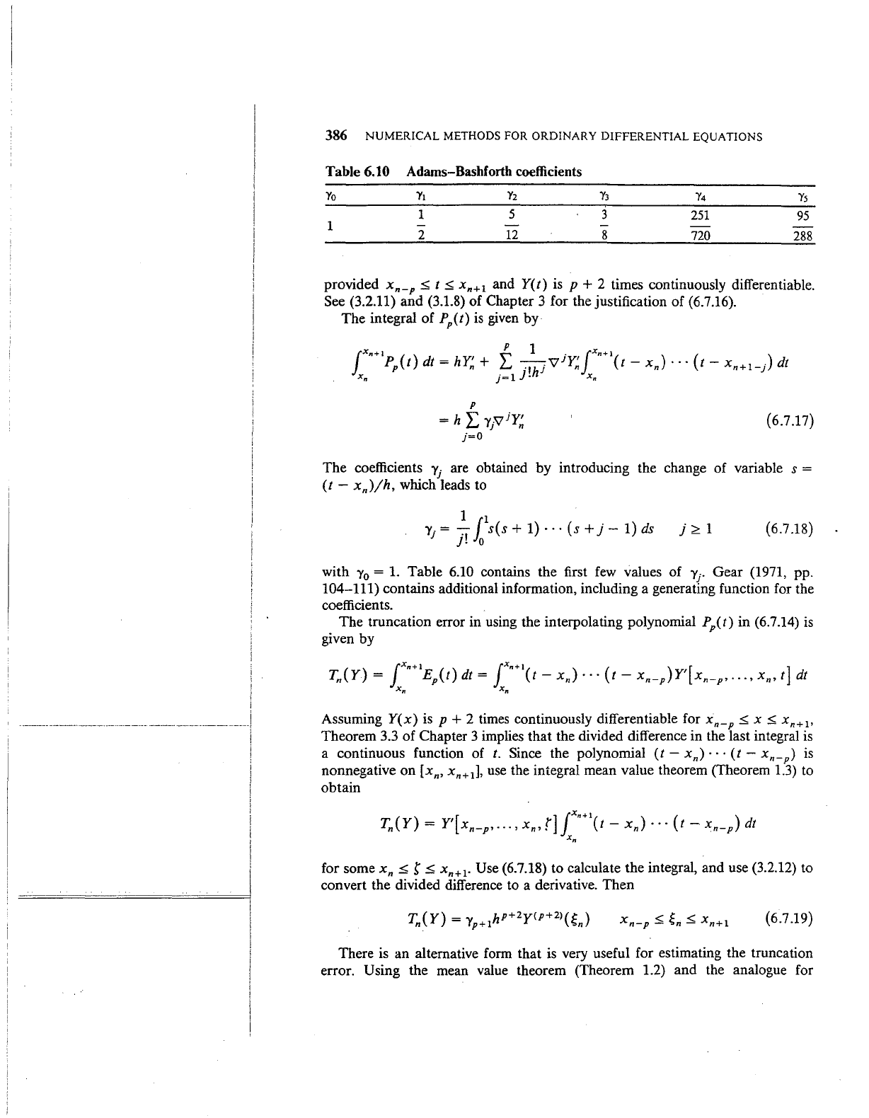
Case
1.
Adams-
Bashforth Methods Let
Pp(
t)
denote the polynomial
of
degree
~
p
that
interpolates
Y'(t)
at
xn-p•
...
, xn. The most convenient form
for PP(t) will
be
the Newton backward difference formula (3.3.11), expanded
about
xn:
(
t
-X
) (t - X
)(t
- X )
p { ) _ Y' n Y' n n-1
2
Y'
...
p t - n + h 'V n + 2!h2 'V n +
(
t-
X ) • • •
(t
- X )
+ n n-p+l PY'
p!hP 'V n
{6.7.15)
As
an
illustration
of
the notation, V
Y~
= Y'(xn) - Y'(xn_
1
),
and
the higher
order backward differences are defined accordingly [see (3.3.10)]. The interpola-
tion error is given by
Ep{t) =
(t-
Xn-p) ·
··
(t-
xn)Y'[xn-p•···•
Xn,
t]
(t-
xn_p)
...
(t-
xJ y<p+2>(n
(p
+ 1)! I
Xn-p
~
~
1
~
Xn+l
{6.7.16)
.
---·---·--·---··--··--···-··--···-
·-------···----·-
···-·-
'
!
386
NUMERICAL
METHODS FOR ORDINARY
DIFFERENTIAL
EQUATIONS
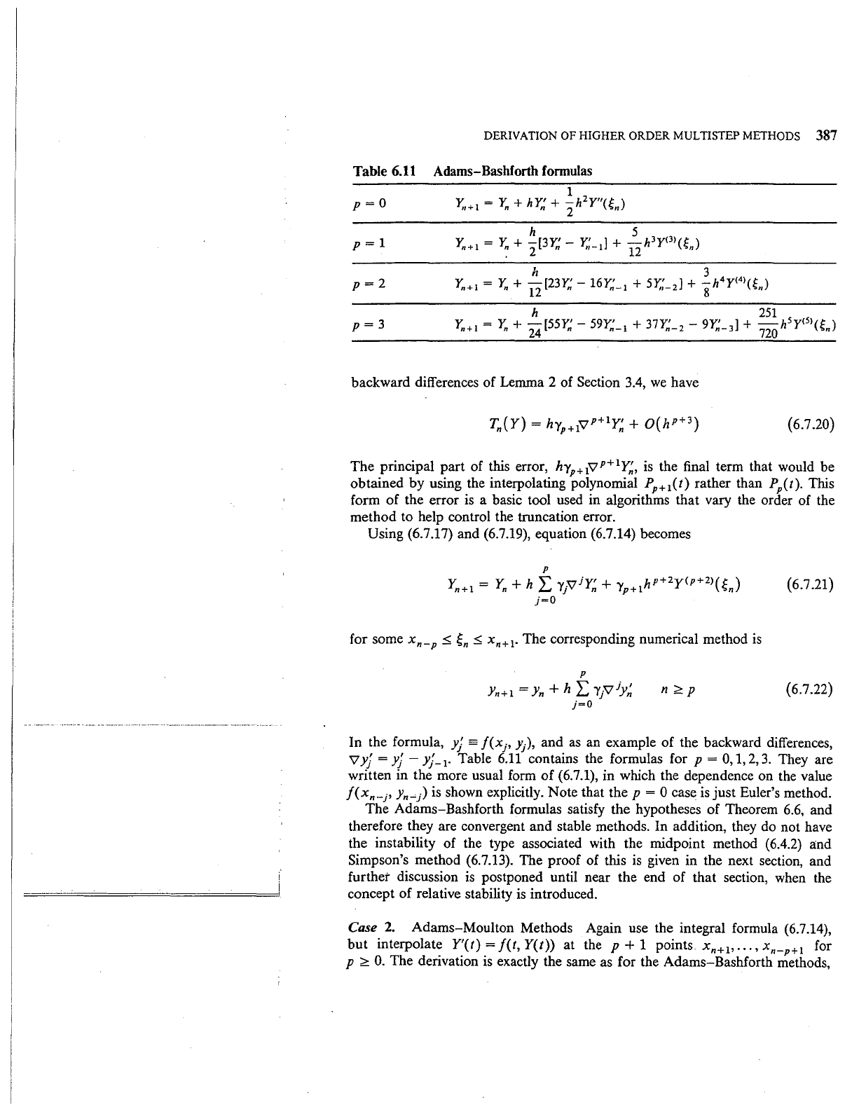
Table 6.10 Adams-Bashforth coefficients
Yo
1
1
2
5
12
3
8
251
720
Ys
95
288
provided xn-p::;:;
t::;:;
xn+l
and Y(t)
is
p + 2 times continuously differentiable.
See (3.2.11) and (3.1.8) of Chapter 3 for the justification of (6.7.16).
The integral of Pp(t)
is
given
by
p
= h
LY]iljY~
j=O
(6.7.17)
The coefficients
Yj
are obtained by introducing the change of variable s =
(t-
xn)fh,
which leads to
1
11
y.
=
-:-
s(s
+
1)
· · · (s +
j-
1)
ds
J
j!
0
}~1
(6.7.18)
with
Yo=
1. Table 6.10 contains the first
few
values of
Yj·
Gear (1971, pp.
104-111) contains additional information, including a generating function for the
coefficients.
The truncation error in using the interpolating polynomial
PP(t) in (6.7.14)
is
given by
Assuming
Y(x) is p + 2 times continuously differentiable for xn-p::;:;
X::;:;
xn+l•
Theorem 3.3
of
Chapter 3 implies that the divided difference in the last integral
is
a continuous function of t. Since the polynomial
(t
-
xn)
· · ·
(t
-
xn-p)
is
nonnegative on [xn,
xn+d,
use the integral mean value theorem (Theorem 1.3) to
obtain
for some
xn
::;:;
t::;:;
xn+l·
Use (6.7.18) to calculate the integral, and use (3.2.12) to
convert the divided difference to a derivative. Then
(6.7.19)
There
is
an alternative form that is very useful for estimating the truncation
error.
Using the mean value theorem (Theorem 1.2) and the analogue for
DERIVATION OF HIGHER ORDER MULTISTEP METHODS 387
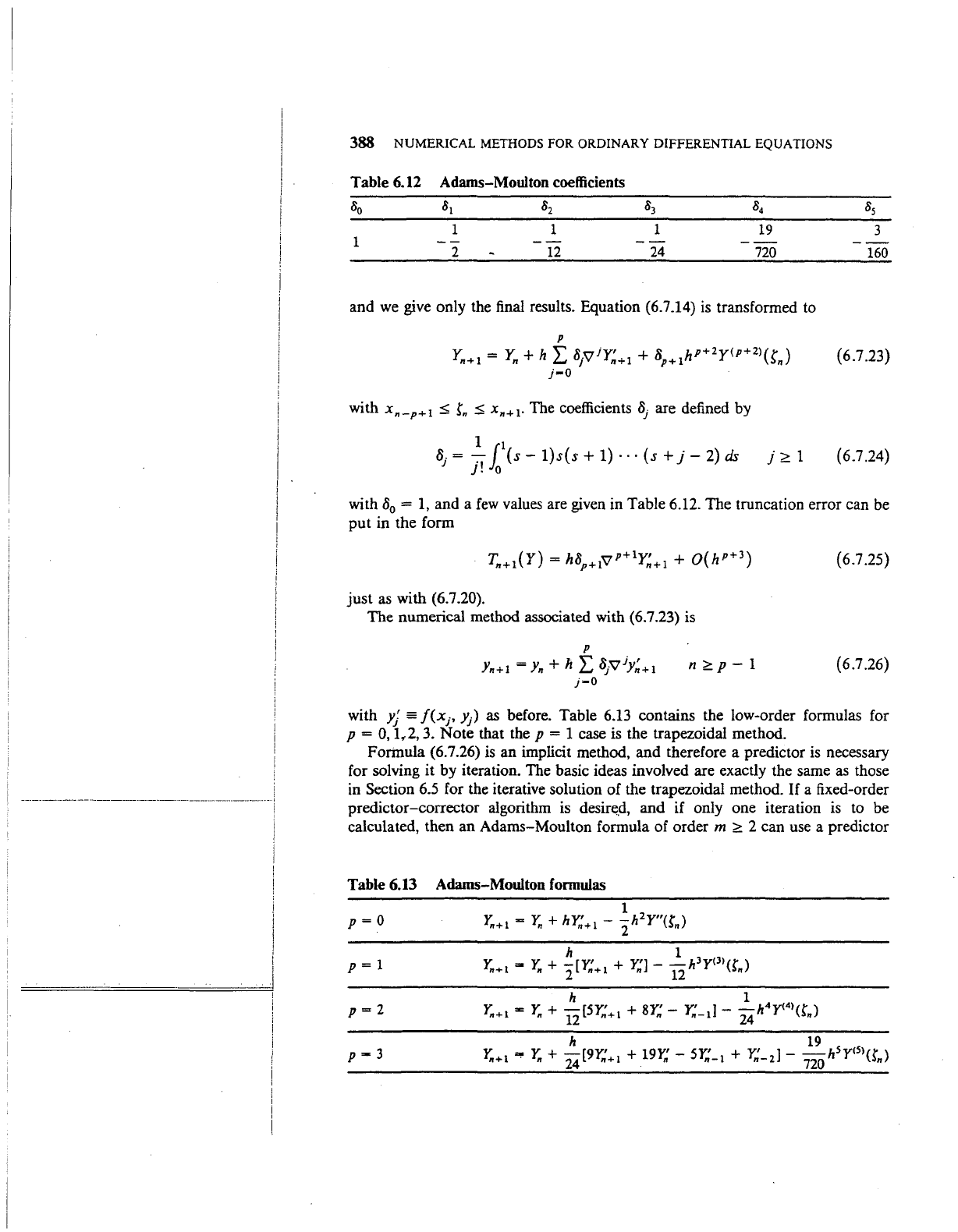
Table
6.11
Adams-Bashforth formulas
backward differences of Lemma 2 of Section
3.4,
we
have
( 6.7.20)
The principal part of this error,
kyp+i'\lp+Iy~,
is
the final term that would be
obtained by using the interpolating polynomial
Pp+
1
(t)
rather than PP(t). This
form
of
the error
is
a basic tool used in algorithms that vary the order of the
method to help control the truncation error.
Using
(6.7.17) and (6.7.19), equation (6.7.14) becomes
for some
xn-p::;;
~n::;;
xn+l· The corresponding numerical method
is
p
Yn+l
=
Yn
+ h L
"Yj'VjY~
j=O
n
?:.
p
(6.7.21)
(6.7.22)
In the formula,
yj
=
f(xj,
y),
and
as
an example of the backward differences,
'\lyj =
yj-
yj_
1
•
Table
6.11
contains the formulas for p =
0,
1,2,3. They are
written in the more usual form
of
(6.7.1), in which the dependence on the value
f(xn-p
Yn~)
is
shown explicitly. Note that the p = 0 case
is
just
Euler's method.
The Adams-Bashforth formulas satisfy the hypotheses of Theorem
6.6, and
therefore they are convergent and stable methods. In addition, they do not have
the instability of the type associated with the midpoint method (6.4.2)
a:nd
Simpson's method (6.7.13). The proof of this
is
given in the next section, and
further discussion
is
postponed until near the end of that section, when the
concept of relative stability
is
introduced.
Case
2.
Adams-Moulton Methods Again use the integral formula (6.7.14),
but interpolate
Y'(t)
=
f(t,
Y(t))
at the p + 1 points.
Xn+l•
...
' xn-p+l for
p
?:.
0.
The derivation is exactly the same
as
for the Adams-Bashforth methods,
388
NUMERICAL METHODS FOR ORDINARY DIFFERENTIAL EQUATIONS
Table 6.12 Adams-Moulton coefficients
8o
8,
82
83 84
85
1 1 1
19
3
1
--
2
12
24
720
160
and
we
give only the final results. Equation (6.7.14)
is
transformed to
p
Y = Y +
h"
8.yriY' + 8
hP+
2
y<P+
2
>("'
)
n+l
n £.. 1
n+l
p+l
~n
( 6.7 .23)
J-0
with
xn-p+l
~
tn
~
xn+l·
The coefficients
8}
are defined by
1
11
8.
=
-:-
(s-
1)s(s +
1)
· · · (s +
j-
2)
ds
1
j!
0
( 6.7 .24)
with
8
0
=
1,
and a
few
values are given in Table 6.12. The truncation error can be
put
in the form
just
as with (6.7.20).
The numerical method associated with (6.7.23) is
p
Yn+l
=
Yn
+ h L
8p
1
y~+l
J-0
n~p-1
( 6.7 .25)
(6.7.26)
with
yj
=
f(x
1
,
Y)
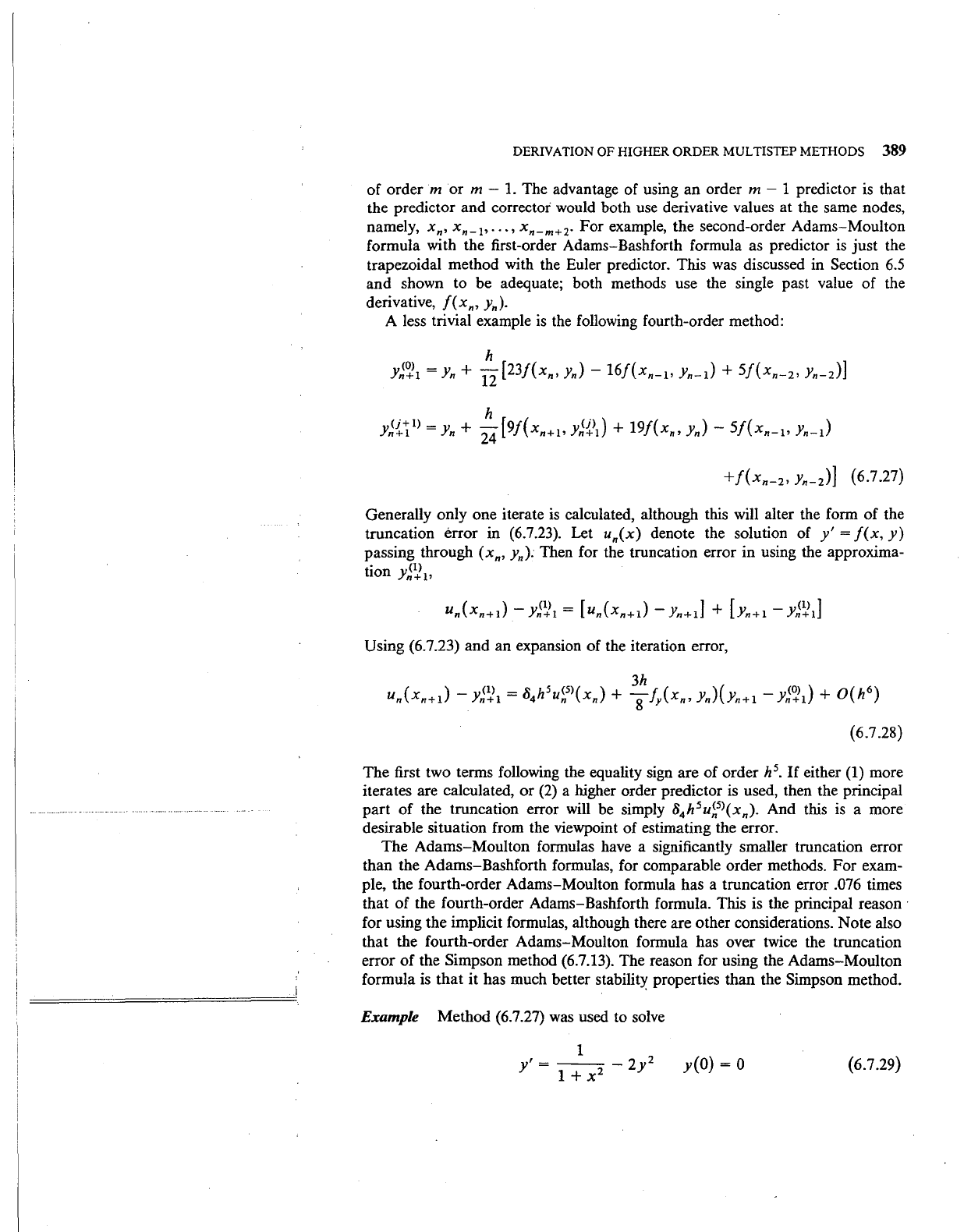
as before. Table 6.13 contains the low-order formulas for
p
=
0,
1~2,
3.
Note that the p = 1 case is the trapezoidal method.
Formula (6.7.26)
is
an implicit method, and therefore a predictor is necessary
for solving it by iteration. The basic ideas involved are exactly the same as those
in Section 6.5 for the iterative solution of the trapezoidal method.
If
a fixed-order
predictor-corrector algorithm is desire.d, and if only one iteration
is
to be
calculated, then an Adams-Moulton formula of order
m
~
2 can use a predictor
Table 6.13 Adams-Moulton fonnulas
DERIVATION OF HIGHER ORDER MULTISTEP METHODS 389
of order m
or
m - 1. The advantage of using an order m - 1 predictor
is
that
the predictor and corrector would both use derivative values at the same nodes,
namely, xn, xn_
1
,
...
, xn-m+
2
. For example, the second-order Adams-Moulton
formula with the first-order Adams-Bashforth formula as predictor
is
just
the
trapezoidal method with the Euler predictor. This was discussed in
Section
6.5
and shown to be adequate; both methods use the single past value of the
derivative,
f(xn,
Yn)·
A less trivial example
is
the following fourth-order method:
h
Y~<::\
=
Yn
+
12
[23/{xn,
Yn)
- 16j(xn-1• Yn-1) +
5j(xn-2•
Yn-2)]
h
y~{~
1
)
=
Yn
+
24
[9J(xn+1•
Y~{>1)
+
19/(xn,
yJ-
5/(xn-1•
Yn-1)
+j(xn-2•
Yn-2)] (6.7.27)
Generally only one iterate
is
calculated, although this will alter the form of the
truncation
error in (6.7.23). Let un(x) denote the solution of
y'
=
f(x,
y)
passing through (xn,
Yn)·
Then for the truncation error in using the approxima-
tion
y~2
1
,
(
)
- {1) - [ ( ) - ]
+ [ - {1) ]
un
xn+1
Yn+!-
un
xn+1
Yn+1
Yn+!
Yn+!
Using (6.7.23) and an expansion
of
the iteration error,
( 6.7 .28)
The first two terms following the equality sign are of order h
5
•
If
either
(1)
more
iterates are calculated,
or
(2)
a higher order predictor
is
used, then the principal
part
of the truncation error will be simply
8
4
h
5
u~
5
>(xn).
And this
is
a more
desirable situation from the viewpoint
of
estimating the error.
The Adams-Moulton formulas have a significantly smaller truncation error
than the Adams-Bashforth formulas, for comparable order methods. For exam-
ple, the fourth-order Adams-Moulton formula has a truncation error
.076 times
that of the fourth-order Adams-Bashforth formula. This is the principal reason·
for using the implicit formulas, although there are other considerations. Note also
that the fourth-order Adams-Moulton formula has over twice the truncation
error of the
Simpson method (6.7.13). The reason for using the Adams-Moulton
formula is
that
it has much better
stabilit~
properties than the Simpson method.
Example Method (6.7.27) was used to solve
1
y'=
--
-2y2
1 + x
2
y(O)
= 0
(6.7.29)
390 NUMERICAL METHODS FOR ORDINARY DIFFERENTIAL EQUATIONS
Table
6.14
Numerical example of the Adams method
Error
for
Error
for
X
h =
.125
h =
.0625
Ratio
2.0
2.07E-
5
1.21E-
6
17.1
4.0
2.21E-
6
1.20E-
7
18.3
6.0
3.74E-
7
2.00E-
8
18.7
8.0
l.OOE-
7
5.24E-
9
19.1
10.0
3.58E-
8
1.83E-
9
19.6
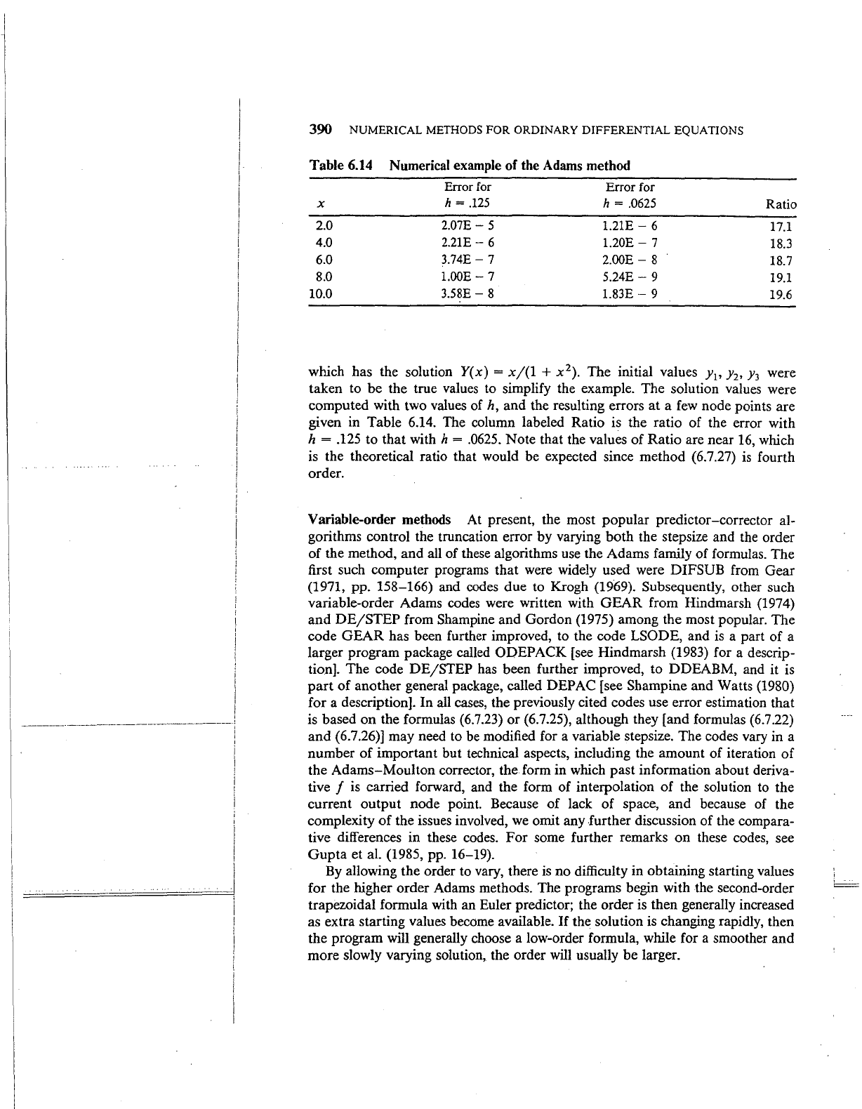
which has the solution
Y(x)
=
x/(1
+ x
2
).
The initial values y
1
,
Jl,
y
3
were
taken to be the true values to simplify the example. The solution values were
computed with two values of
h, and the resulting errors
at
a
few
node points are
given in Table 6.14. The column labeled Ratio is the ratio of the error with
h = .125 to that with h =
.0625.
Note that the values of Ratio are near
16,
which
is
the theoretical ratio that would be expected since method {6.7.27)
is
fourth
order.
Variable-order methods At present, the most popular predictor-corrector al-
gorithms control the truncation error by varying both the stepsize and the order
of the method, and all of these algorithms use the Adams
family of formulas. The
first such computer programs that were widely used were DIFSUB from Gear
(1971, pp. 158-166) and codes due to Krogh (1969). Subsequently, other such
variable-order Adams codes were written with
GEAR
from Hindmarsh (1974)
and
DE/STEP
from Shampine and Gordon (1975) among the most popular. The
code
GEAR
has been further improved, to the code LSODE, and
is
a part of a
larger program package called
ODEPACK [see Hindmarsh (1983) for a descrip-
tion]. The code
DE/STEP
has been further improved, to DDEABM, and it is
part
of another general package, called DEPAC [see Shampine and Watts (1980)
for a description]. In all cases, the previously cited codes use error estimation that
is based on the formulas (6.7.23)
or
(6.7.25), although they [and formulas (6.7.22)
and (6.7.26)] may need to be modified for a variable stepsize. The codes vary in a
number
of
important but technical aspects, including the amount of iteration
of
the Adams-Moulton corrector, the form in which past information about deriva-
tive
f
is
carried forward, and the form of interpolation of the solution to the
current output node point. Because of lack of space, and because of the
complexity
of
the issues involved,
we
omit any .further discussion of the compara-
tive differences in these codes. For some further remarks
on
these codes, see
Gupta
et al. (1985, pp. 16-19).
By
allowing the order to vary, there
is
no difficulty in obtaining starting values
for the higher order Adams methods. The programs begin with the second-order
trapezoidal formula with an Euler predictor; the order
is
then generally increased
as extra starting values become available.
If
the solution
is
changing rapidly, then
the program will generally choose a low-order formula, while for a smoother and
more slowly varying solution, the order will usually be larger.
